1. Quick Start
Expressions can be used in query filters, for result sorting, and to select result fields. Below are three examples showing each case.
1.1. filter
This filter requires the value of the arc from "A" to its neighbor to be greater than 10 and the neighbor id must equal "B" or start with "C" or end with "d".
graph.Neighborhood( "A",
    filter=".arc.value > 10 && next.id in {'B', 'C*', '*d'}"
)
1.2. rank
This custom ranking function will divide the neighbor’s "score" property by the arc value and multiply the result by the anchor’s "boost" property. The function’s output value is used for sorting the query results.
graph.Neighborhood( "A",
    rank="vertex['boost'] * (next['score'] / .arc.value)",
    sortby=S_RANK
)
1.3. select
This select statement formats the query result to include the neighbor’s "score" property, the value of the arc from "A" to its neighbor, and a computed value with custom name "RATIO".
graph.Neighborhood( "Alice",
    select="score; .arc.value; RATIO: next['score'] / .arc.value"
)
See Select Evaluator for details.
1.4. Quick Reference
| Section | Description | ||
|---|---|---|---|
Define an expression and assign it to a name |
|||
Evaluate an expression |
|||
Expression syntax and operators |
|||
→ |
Arc attributes (relationship type, value, etc.) |
||
→ |
Vertex attributes (id, degree, timestamps, etc.) |
||
→ |
User defined vertex properties (key/value pairs) |
||
Pre-defined numeric constants for use in expressions |
|||
Variables derived from current execution environment |
|||
→ |
Basic math functions ( |
||
→ |
Check and convert data types ( |
||
→ |
Basic string operations ( |
||
→ |
Retrieve vertex property by key |
||
→ |
Encode or decode enumerations ( |
||
→ |
Compute vector similarity ( |
||
→ |
Control functions ( |
||
→ |
Aggregate multiple variable arguments ( |
||
→ |
Basic functions for ranking search results ( |
||
→ |
Collect result data in expressions ( |
||
→ |
These functions perform operations on a specified memory location |
||
Write and read memory data location ( |
|||
Memory stack operations ( |
|||
Move data between memory locations ( |
|||
Inc/dec data in memory location ( |
|||
Compare data in two memory locations ( |
|||
Arithmetic operations on memory location ( |
|||
Bitwise operations on memory location ( |
|||
AVX accelerated bytearray vector operations ( |
|||
Smoothing and counting ( |
|||
Various memory indexing helper functions ( |
|||
→ |
These functions perform array operations on multiple memory locations |
||
Assign and copy data ( |
|||
Min/max-heap operations ( |
|||
Sort a memory range ( |
|||
Convert data in multiple memory locations ( |
|||
Inc/dec all locations in memory range ( |
|||
Arithmetic on multiple memory locations ( |
|||
Numeric operations on multiple locations ( |
|||
Apply log/exp to memory range ( |
|||
Apply trig/hyp functions to memory range ( |
|||
Bit shift and logical operations on memory range ( |
|||
Hash multiple memory locations ( |
|||
Aggregate memory range ( |
|||
Search memory range ( |
|||
→ |
|||
|
|||
|
|||
2. Overview
VGX has a built-in evaluator engine for executing user-defined expressions. Custom formulas can be used in traversal filters (filter=), result ranking (rank=) and rendering of selected fields (select=). For example:
graph.Neighborhood(
    "Alice",
    filter  = "next.id in {'B*','*ch*'}",
    rank    = "next.arc.value / next['age']",
    select  = ".id; age",
    sortby  = S_RANK
)
The expression syntax supports grouping, nesting, logical operators, comparison operators, property lookup, array indexing, membership tests for discrete and continuous sets, and all the standard mathematical operators and functions. Expressions can be pre-defined and referenced by name in graph queries.
A comprehensive library of functions, constants and environment variables is available for use in expressions.
It is possible to define and pass a memory array object to queries. Expressions evaluated as part of a query may then read or write elements of the memory array, opening up many possibilities for algorithm design. For instance, variables captured by a filter expression may be passed as input to a ranking expression. The same memory array object can be used by different queries enabling information sharing from one query to the next. Other uses include value aggregation, creating histograms, tracking graph cycles, and computing averages or deviations just to name a few.
Expressions can also be evaluated stand-alone using pyvgx.Graph.Evaluate(). For example:
graph.Evaluate( "1+1" ) # -> 2
graph.Evaluate( "log( (2.1e3 + 4.5) * (pi - sin(6.7)) )" ) # -> 8.66...
2.1. Safe Evaluation
Due to the schemaless and dynamic nature of data values encountered during traversal the evaluator uses a best-effort approach when computing results. In general the evaluator will compute expressions "the way you intended." Where it deviates from many programming languages is in the lenient handling of operations on incompatible objects, zero division, domain errors, accessing non-existent properties, and out of range array indices.
It is impossible to write an expression that will crash, lock or leave the system in a corrupted state.
2.1.1. Incompatible Objects
Operations on incompatible objects will generally produce results as if the operations were not performed, which usually means keeping the leftmost operand. For example, "5 / 'a string'" will produce 5 and "5 / 'a string' + 1" will produce 6.
2.1.2. Divide by Zero
The result of zero division is generally a "very large number". For example, 1/0 evaluates to 8.5e37. This interpretation of zero division ensures formulas are computable even as divisors approach (and reach) zero. The divisor -0.0 is an exception in that 1/-0.0 produces -inf and 0/-0.0 produces nan.
2.1.3. Domain Errors
Some mathematical functions accept arguments outside their defined domains. Roots of negative numbers produce zero (imaginary numbers are not supported.) Logarithms of zero or negative numbers produce a negative number which depends on the base. For example sqrt(-1) evaluates to 0, log(0) evaluates to -745.0 and log2(-1) evaluates to -1074.0. Computation involving roots and logarithms will always produce numeric results.
Other functions, such as the trigonometric functions, will produce nan for invalid arguments. For instance, asin(2) results in nan as does sqrt(-1) + asin(2) + 5.
2.1.4. Non-existent Vertex Properties
Lookup of a non-existent property will be processed as if the lookup did not take place. For example, if property "x" does not exist then 1 + vertex['x'] + 2 evaluates to 3 and 5 / vertex['x'] evaluates to 5, even though isnan( vertex['x'] ) yields true.
Following this logic, cos( vertex['x'] ) is nan while both 1 + cos( vertex['x'] ) and cos( 0 + vertex['x'] ) return 1.
Default values for non-existent properties can be obtained in two ways. The first method is function vertex.property( "x", default ) which returns property "x" of current tail (i.e. vertex['x']) if it exists, or default if the property does not exist. The second method is function firstval(), which is variadic (i.e. any number of arguments) and returns the leftmost argument that is not nan. For example, firstval( vertex['x'], 2.5 ) returns 2.5 if property "x" does not exist and firstval( next['x'], asin(next['y']), pi/2 ) returns Π/2 if the two preceding arguments both produce nan.
Substitute next or prev for vertex to access properties of the current head or previous tail when traversing arcs. E.g. next.property( x ) or prev.property( x ).
|
2.1.5. Out of Range Subscripts
Operations involving array subscripts employ modulo indexing which guarantees safety. For example, if Evaluator Memory is used and the memory array object has 128 slots store(5, 100), store(133, 100), and store(-123, 100) are equivalent; they all assign value 100 to memory location 5. The size of memory array objects is always a power of two. The last four slots are aliased with registers R1, R2, R3 and R4. There is also a stack which grows downward starting at the slot just before the registers. It is the responsibility of the programmer to ensure algorithm correctness and avoid undesired modulo indexing or aliasing conflicts between array subscripts, registers, and stack.
2.2. Data Types
The evaluator engine can operate on objects of various types. If a function is called with an incompatible argument the result is generally the unprocessed argument, such as sin('hello') which simply returns 'hello'.
Many operators and functions automatically adjust their behavior according to the argument types. For example, the function hash() produces a 64-bit integer hash of the argument, which can be of any type, but uses different algorithms depending on the type. (hash( 123 ), hash( 'hello' ) and hash( vector ) are all valid.)
The final result of an expression is interpreted according to the context where it appears. Filters are concerned with matching (positivity), ranking is concerned with numeric scores and select statements expect lists of objects to render.
| Type | Positive Match | As Rank Score | Type Check | Description |
|---|---|---|---|---|
> 0 |
real( self ) |
64-bit signed integer. |
||
> 0.0 |
self |
64-bit (double precision) floating point. |
||
true |
real( first_5_bytes_as_int ) |
Text string or raw bytes. May appear as function argument or return value. |
||
first item |
first item value |
Comma separated list of objects |
||
(N/A) |
(N/A) |
Continuous set of numbers from a to b |
||
false |
0.0 |
Discrete set of objects |
||
true |
real( address ) |
Object of type <vector> |
||
!= 0 |
real( self ) |
64-bit unsigned integer for use with certain operations that handle bit masks and integers differently. |
||
value > 0.0 |
value |
2-tuple (key, value) where key is a 32-bit signed integer and values is a single precision float. |
||
true |
real( address ) |
Object of type pyvgx.Vertex |
||
true |
real( address ) |
The identifier string of an object of type pyvgx.Vertex |
||
false |
0.0 |
Not a number |
||
false |
0.0 |
No value |
||
true |
0.0 |
Infinity |
2.2.1. Type integer
graph.Evaluate( "1000" )   # -> 1000
graph.Evaluate( "-1000" )  # -> -1000
graph.Evaluate( "01000" )  # -> 1000   leading zeros ignored
graph.Evaluate( "0x1000" ) # -> 4096   0x prefix for hexadecimal
graph.Evaluate( "0X1000" ) # -> 4096   0X also accepted
graph.Evaluate( "0xffffffffffffffff" ) # -> -1   2's complement
graph.Evaluate( "0xfffffffffffffffe" ) # -> -2   2's complement
2.2.2. Type real
graph.Evaluate( "3.14" )  # -> 3.14
graph.Evaluate( ".123" )  # -> 0.123
graph.Evaluate( "1e3" )   # -> 1000.0
graph.Evaluate( "-.1e1" ) # -> 1.0
2.2.3. Type string
graph.Evaluate( "'hello'" ) # -> 'hello'2.2.4. Type group
graph.Evaluate( "(1,2,3,4)" ) # -> 1
graph.Evaluate( "('hello',2,3,4)" ) # -> 'hello'
2.2.5. Type range
graph.Evaluate( "0.999 in range(1,3)" ) # -> 0
graph.Evaluate( "1 in range(1,3)" ) # -> 1
graph.Evaluate( "2.999 in range(1,3)" ) # -> 1
graph.Evaluate( "3 in range(1,3)" ) # -> 0
2.2.6. Type set
graph.Evaluate( "{1, 2, 3}" ) # -> '<set>'
graph.Evaluate( "2 in {1, 2, 3}" ) # -> 1
graph.Evaluate( "2.999 in {1, 2, 3}" ) # -> 0
2.2.7. Type vector
X = graph.NewVertex( "X" )
Y = graph.NewVertex( "Y" )
X.SetVector( [('a',1),('b',0.5),('c',0.25)] )
Y.SetVector( [('a',1),('b',0.75),('c',0.5)] )

E = graph.Evaluate

### Vector type
E( "next.vector", head="X" ) # -> '<vector>'

### Length
E( "len( next.vector )", head="X" ) # -> 3

### Magnitude
E( "asreal( next.vector )", head="X" ) # -> 1.14564394951

### Fingerprint
E( "hash( next.vector )", head="X" ) # -> -3579455383477239039

### Address
E( "int( next.vector )", head="X" ) # -> 2337927647264

### Element of
E( "'c' in next.vector", head="X" ) # -> 1
E( "'d' in next.vector", head="X" ) # -> 0

### Similarity
g.Evaluate( "sim( prev.vector, next.vector )", tail="X", head="Y" ) # -> 0.97265625
2.2.8. Type bitvector
graph.Evaluate( "0b11110000" ) # -> '<bitvector 0x00000000000000f0>'2.2.9. Type keyval
graph.Evaluate( "keyval(1000,0.5)" ) # -> '<keyval (1000,0.5)>'

### Key
graph.Evaluate( "int( keyval(1000,0.5) )" ) # -> 1000

### Value
graph.Evaluate( "real( keyval(1000,0.5) )" ) # -> 0.5
2.2.10. Type vertex
V = graph.NewVertex( "Node1" )
V['x'] = 1000
graph.Connect( "Node1", "to", "X" )
graph.Connect( "Node1", "to", "Y" )

### Attribute
graph.Evaluate( "next.odeg", head=V ) # -> 2
graph.Evaluate( "next.tmc", head=V ) # -> 1642822680

### Internalid string
graph.Evaluate( "str(next)", head=V ) # -> '76fd13f0d0135ed4c7ed813e1c3db986'

### Address
graph.Evaluate( "int( next )", head=V ) # -> 2336660804768

### Property
graph.Evaluate( "int( next )", head=V ) # -> 2336660804768
graph.Evaluate( "'x' in next", head=V ) # -> 1
graph.Evaluate( "'y' in next", head=V ) # -> 0
graph.Evaluate( "next['x']", head=V ) # -> 1000
2.2.11. Type vertexid
V = graph.NewVertex( "Node1" )
graph.Evaluate( "next.id", head=V ) # -> 'Node1'
hex(graph.Evaluate( "hash( next.id )", head=V )) # -> '-0x38127ec1e3c2467a'
2.2.12. Type nan
graph.Evaluate( "nan" ) # -> nan
graph.Evaluate( "acos(2)" ) # -> nan  # domain error
graph.Evaluate( "acos(2) == nan" ) # -> 1
graph.Evaluate( "1.8e308" ) # -> nan  # out of range
2.2.13. Type null
graph.Evaluate( "null" )
graph.Evaluate( "isnan( null )" ) # -> 1
2.2.14. Type inf
graph.Evaluate( "inf" ) # -> inf
graph.Evaluate( "1e300 * 1e300" ) # -> inf
graph.Evaluate( "1e300 * 1e300 == inf" ) # -> 1

### Infinity is considered numeric
graph.Evaluate( "isnan( inf )" ) # -> 0

### NOTE: The expression language is designed to produce
###       numeric results even when infinity is involved
###       in the computation. Dividing by zero produces
###       "a very large number" and dividing by infinity
###       produces zero.
graph.Evaluate( "1/inf" ) # -> 0.0
graph.Evaluate( "1**inf" ) # -> 1.0
graph.Evaluate( "1.000001**inf" ) # -> 1.7976931348623157e+308
graph.Evaluate( "0.999999**inf" ) # -> 0.0
graph.Evaluate( "inf/inf" ) # -> nan
graph.Evaluate( "inf-inf" ) # -> nan
graph.Evaluate( "-1/-0.0" ) # -> inf # Special case
graph.Evaluate( "-1/-0.0 == inf" ) # -> 1
2.3. No Short Circuiting
There are no short-circuit operators, leaving no doubt about which parts of expressions are evaluated: all sub-expressions within a complex expression are always executed.
For example "1 > 2 && inc( R1 ) > 10" will naturally always be false (due to 1 > 2 part), but will regardless execute inc( R1 ).
| This behavior is different from many programming languages, so beware. |
Conditional execution requires explicit use of a conditional function. The above example may be rewritten to perform operations conditionally (also replacing 1 > 2 with the more useful .arc.value > 2), like this:
"incif( .arc.value > 2, R1 ) && load( R1 ) > 10". Here the value in register R1 is only incremented when .arc.value > 2 and the entire expression evaluates to true after 11 iterations where the .arc.value condition was met.
Be careful when writing filters to avoid unintended overhead in computation and memory access.
There are exactly two exceptions to the no short-circuiting execution policy. The functions return() and returnif() can be placed within an expression to terminate execution at that point in the expression.
2.4. Expression Examples
Suppose we have created a graph with relationships between friends. The following examples show how we can filter, rank results and select fields to return.
2.4.1. Filter Example
graph.Neighborhood(
    "Alice",
    filter  = "( .arc.type in {'friend','knows','likes'} && .type == 'person' ) || ( .arc.type == 'owns' && .type == 'pet' )"
)
Here we use filter= to match three different relationships ("friend", "knows", or "likes") using the in { … } set operator and combine sub-expressions with boolean operators && and ||.
Complex matching logic like this is not possible using arc= and neighbor= parameters alone. However, in many cases it may be more efficient to also include arc= and neighbor= in the query, since they may help reduce the amount of processing performed by the expression evaluator by early termination of non-matching filters.
|
2.4.2. Dynamic Ranking Example
graph.Neighborhood(
    "Alice",
    sortby = S_RANK,
    rank   = ".arc.value * ( 1 + 9 * (.arc.type == 'friend')) / next.deg"
)
Here we use rank= to specify a custom scoring function. To use the computed scores for sorting results we must also specify sortby=S_RANK. In this example results are ordered according to arc values divided by neighbor’s degree, boosting relationships of type 'friend' by a factor 10.
2.4.3. Select Result Fields Example
graph.Neighborhood(
    "Alice",
    select = "age; address; SCORE1: .arc.value / (1 + log( next.odeg / next.ideg )); LABEL1: hash( next.id )"
)
The select statement specifies a semicolon-separated list of items to return. Items can be attributes, vertex properties, or computed values identified by labels. If the item is a single token it is interpreted as a vertex property key, unless it starts with a period "." which is interpreted as an attribute (such as ".id" which is short for "next.id").
When the item is a labeled expression "label : …" any valid expression can be specified to dynamically compute values. The computed values will be identifiable in the result by their labels.
This example includes Alice’s neighbors' age, address, some computed number identified by label SCORE1, and another computed value identified by LABEL1.
3. Expression Language Reference
Expressions are constructed using syntax similar to many programming languages, and offer a wide variety of built-in function. The following sections summarize all available symbols, functions and constructs.
Expressions are available to use in query parameters filter=, rank= and select=.
3.1. Define Functions with Define()
An expression may be defined and stored in the graph for future use.
3.1.1. Syntax
pyvgx.Graph.Define( expression )-
Create a new function formula that can be used by queries for filtering and ranking. The expression parameter is a string of the form
<name> := <formula>.
3.1.2. Parameters
| Parameter | Type | Description |
|---|---|---|
expression |
str |
Expression definition of the form |
3.1.3. Return Value
This method does not return anything.
3.1.4. Remarks
Pre-defined expressions are stored in the graph object on which the Define() method was invoked. Expressions defined for a graph instance are exclusive to that instance and cannot be referenced by other graphs.
It is recommended to pre-define complex functions before using them in queries since parsing and compiling occur only when the expression is defined. Eliminating this overhead may help speed up query execution, and in cases where the same expression is used by multiple queries it is easier to maintain consistent functionality.
| Make sure type enumerations exist for all arc relationship types and vertex types that appear in the expression before the expression is defined. Otherwise the expression will not be correctly evaluated. |
3.2. Evaluate Expressions with Evaluate()
An expression may be evaluated outside the context of a query for testing or for operations that do not require a graph query.
3.2.1. Syntax
pyvgx.Graph.Evaluate( expression[, tail[, arc[, head[, vector[, memory ]]]]] )-
Execute the expression, which is a string defining a new formula, or referencing a pre-defined formula. The optional parameters are used to supply information that may be referenced in the formula.
3.2.2. Parameters
| Parameter | Type | Default | Description |
|---|---|---|---|
expression |
str |
Expression to be evaluated |
|
tail |
str or pyvgx.Vertex |
None |
Vertex whose attributes and properties may be accessed via the various |
arc |
() |
Arc whose attributes may be accessed via the various |
|
head |
str or pyvgx.Vertex |
None |
Vertex whose attributes and properties may be accessed via the various |
vector |
<vector> or Python list |
[] |
Similarity vector which may be accessed via the |
memory |
pyvgx.Memory or int |
4 |
Memory array object which may be accessed using the various memory operations. |
3.2.3. Return Value
This method returns the result of the evaluation, which may be an integer, a floating point object (including nan or inf), a string, or other object.
3.2.4. Remarks
This method is useful for experimenting with expressions before using them with queries. It can also be used for pre/post processing memory arrays outside the context of a query. For example, if a query was used to gather information into a memory array object this method can then be used to access and further process that information.
All processing within the evaluator occurs outside the Python interpreter, allowing for multi-threaded operation and in some cases more efficient single-threaded processing. For instance, running msum() on a large memory array of 100,000,000 floating point numbers is about 5 times faster than Python’s native sum() function on an equivalent Python array. Moreover, running mradd() on the same memory array is about 50 times faster than performing the equivalent operation in a pure Python loop.
3.3. Basic Expression Syntax
Expressions are evaluated according to operator precedence and associativity, as commonly used in most programming languages. The table below summarizes the syntax rules.
3.3.1. Group
Operations may be enclosed in parentheses ( ) to override default precedence rules. Groups may be nested to construct any mathematical formula or logical expression. Nesting is unlimited.
1 / ( ( 2 + 3 ) * ( 4 + 5 ) ) // -> 0.02222...A group can also be used to perform one or more "hidden" operations needed for their side-effects. When multiple expressions separated by comma , appear within the group only the value of the first expression becomes the value of the group. All subsequent expressions are evaluated but their return values are discarded.
( 1, 2, 3 ) + ( 1.5, 2.5, 3.5 )                 // -> 2.5
10 * ( 2, store( R1, pi ) )                     // -> 20
4 ** 3 - 2 + 1                                  // -> 63
4 ** (3 - 2) + 1                                // -> 5
4 ** 3 - (2 + 1)                                // -> 61
4 ** (3 - 2 + 1)                                // -> 16
3.3.2. Set
A set of discrete numbers or objects is created by placing them within braces { }, items separated by commas ,.
{ 3, 4, 5, 'hello', 6.7 }3.3.3. Function Call
A pair of parentheses (…) with optional comma , separated arguments is interpreted as a function call when the preceding token is a string.
random()
log( 1.23 )
mmul( 0, 31, pi )
3.3.4. Subscript
A literal string 's' within a pair of brackets [ 's' ] denotes a property lookup when the preceding token is a vertex object. Properties are readonly.
vertex[ 'prop1' ]
next[ 'value' ]
3.3.5. Attribute
The dot . operator is used to access vertex attributes, arc attributes and various context information. Attributes are readonly.
vertex.id
next.arc.value
graph.size
3.3.6. Unary Plus/Minus
Unary plus + and minus − set the sign of a numeric value.
-1                      // -> -1
-(+2 - +5)              // -> 3
-7+-1--8                // -> 0
3.3.7. Logical NOT
The exclamation point ! negates a logical value.
!0                      // -> 1
!1                      // -> 0
!2                      // -> 0
!( true || false )      // -> 0
!( !true || false )     // -> 1
3.3.8. Bitwise NOT
A tilde ~ denotes one’s complement of a numeric value, i.e. all bits are inverted.
~0                      // -> -1
~1                      // -> -2
~0xffffffffffffffff     // -> 0
3.3.9. Exponentiation
A pair of infix asterisks ** raises a number to the power of another number.
16 ** 2                 // -> 256
100.0 ** 0.5            // -> 10.0
e ** -0.1               // -> 0.9048...
3.3.10. In Numeric Range
The in and notin operators followed by range( a, b ) express the numeric range conditions ∈ [ a, b > and ∉ [ a, b >, respectively.
5 in range( 2, 6 )          // -> true
5 in range( 2, 5 )          // -> false
pi in range( 3.1, 3.2 )     // -> true
10 notin range( 1, 5 )      //  -> true
3.3.11. Member of Set
The in and notin operators followed by set { x1, x2, …, xn } express the discrete set membership conditions ∈ { x1, x2, …, xn } and ∉ { x1, x2, …, xn }, respectively.
5 in { 9, 5, 'cat', 'dog' }                 // -> true
4 in { 9, 5, 'cat', 'dog' }                 // -> false
'cat' in { 9, 5, 'cat', 'dog' }             // -> true
'mouse' notin { 9, 5, 'cat', 'dog' }        // -> true
'mouse' in { '*ous*', 'm*e' }               // -> true
'mice' in { '*ous*', 'm*e' }                // -> true
3.3.12. Multiplication
Infix * multiplies two numbers.
2 * 3           // -> 6
2 * pi          // -> 6.28...
3.3.13. Division
Infix / divides a number by another.
15 / 3              // -> 5
16 / 3              // -> 5.33...
3.14 / pi           // -> 0.999...
1 / 0               // -> 8.51e37
1 / -0.0            // -> -inf
When integer division has a remainder the result is promoted to floating point. Zero division results in a large floating point value except for the special case divisor -0.0 which produces -inf.
|
3.3.14. Modulo
Infix % yields the remainder after dividing two numbers.
15 % 3              // -> 0
16 % 3              // -> 1
3.14 % pi           // -> 3.14
6.2 % pi            // -> 3.06...
1 % 0               // -> 0
1.1 % 0             // -> 1.18e-38
1 % -0.0            // -> nan
Modulo zero results in 0 (or very close to 0) except for the special case divisor -0.0 which produces nan.
|
3.3.15. Addition
Infix + adds two numbers or concatenates a string with another object implicitly cast to string.
1 + 1               // -> 2
pi + e              // -> 5.8599...
'x' + 'y'           // -> "xy"
'x' + pi            // -> "x3.14159"
3.3.16. Subtraction
Infix - subtracts a number from another.
1 - 2               // -> -1
pi - e              // -> 0.42331...
3.3.17. Bitwise Shift
Infix << and >> perform left and right bit shift, respectively, of the integer representation of the left operand by the amount specified by the right operand. Bits are not rotated, i.e. once bits are shifted off the left or right edge they are discarded.
1 << 10             // -> 1024
1.9 << 10           // -> 1024
1.9 << 10.0         // -> 1.9
0xff >> 5           // -> 7
0xff >> 40 // -> 0| If the right operand is not an integer the shift operation is not performed. |
3.3.18. Comparison
The infix comparison operators ==, !=, >, >=, <, <= compare the left and right operands yielding true or false. Operands may be numbers, strings, vertices or vectors.
'hello' == '*llo'           // -> true
'cat' != 'dog'              // -> true
5 > 4                       // -> true
5 >= 5.0                    // -> true
5.0 < 4.5                   // -> false
5 <= 4.9999999              // -> false
5 == 4.9999999              // -> true
Two floating point values compare equal when their difference is smaller than approximately 1.1921e-7. This affects == and !=, but not >= and <=.
|
3.3.19. Bitwise Logic
Infix operators &, | and ^ perform bitwise AND, OR and XOR, respectively, on their left and right operands.
0xf0 & 0x3c                 // -> 0x30
0xf0 | 0x3c                 // -> 0xfc
0xf0 ^ 0x3c                 // -> 0xcc
3.3.20. Logical Condition
Infix conditional operators && and || apply the logical conditions AND and OR, respectively, to their left and right operands.
1 == 2 && 2 > 1             // -> false
1 == 2 || 2 > 1             // -> true
1 == 2 && store( R1, 777 ) // -> false (777 still stored in R1)| Logical short circuiting is not applied. All parts of an expression are always evaluated regardless of whether or not they contribute to the overall result of the expression. |
3.3.21. Ternary Conditional
The infix ?: operator selects the second or third operand depending on the value of the first operand.
1 < 2 ? 3 + 4 : 5 + 6                      // -> 7
1 > 2 ? 3 + 4 : 5 + 6                      // -> 11
1 < 2 ? store( R1, 33 ) : store( R1, 44 )  // -> 33  (R1 contains 44)
1 > 2 ? store( R1, 33 ) : store( R1, 44 ) // -> 44 (R1 contains 44)| Logical short circuiting is not applied. All operations are completely evaluated, left to right, regardless of condition. |
3.3.22. Expression definition
The assignment operator := associates a definition with a name that can be referenced later to invoke the expression. Expressions are normally assigned to names using pyvgx.Graph.Define(). However, it is also possible to dynamically assign expressions to names during query execution and then reference those names in other parts of the same query.
func := next['score'] / (10 * .arc.value)
quad := load( R2 ) ** 2 + load( R1 ) + vertex['offset']| Each graph instance has its own expression name scope and expressions cannot be shared between separate graph instances. Assigning an expression to a name will overwrite any previous assignment to that name. |
3.3.23. Sub-expressions and Local Variables
An expression may contain one or more independent sub-expressions separated by semicolons ;. The last sub-expression determines the value of the overall expression. It is optional to terminate the last expression with a semicolon.
It is possible to assign the result of a sub-expression to a local variable. The scope of such a variable extends from the point of assignment until the end of the expression. Variable assignment uses the = operator, and must appear directly after the variable name at the start of a sub-expression. Variable names can be freely chosen so long as they conform to valid key syntax and do not conflict with pre-defined names or functions like pi, e, next, sqrt, etc.
1; 5 + log(10); 2.5;                          // -> 2.5
store(R1, 7); 3 + load( R1 );                 // -> 10
a = 2*pi; b = rad(360); a / b;                // -> 1.0
pi = 3.14; //==> Syntax Error: invalid variable assignment| Variable scope is local to the current evaluation of the expression. Once the last sub-expression has completed and returned its result all variables go out of scope. Use Evaluator Memory for global scope and to transfer data between different expressions or repeated evaluations of the same expression. |
3.3.24. Label
The label operator : is exclusive to select statements, allowing processing of rendered result values to take place and making those values identifiable by the label.
val1: 1 / .arc.value; val2: next['score'] & 0xFFFF; val3: graph.ts
This syntax is only available in select= and the expression cannot be pre-defined.
|
3.3.25. Comma
The comma , is used to separate multiple objects such as function arguments, set members, and group elements.
max( next['score'], vertex['score'] )
next.id in { 'Alice', '*lie', 'B*' }
( .arc.value, inc( R1 ) ) * firstval( next['score'], 1.0 )
x = next['score'] * pi, y = 1 / .arc.value
3.3.26. Semicolon
The semicolon ; is used to terminate sub-expressions within a larger expression, and to separate fields or labeled expressions in select= statements.
/* Sub-Expression */
x = next['score'] / next.degree; y = log(x) + x/2; z = log2( y * x );

/* Select Statement */
.id; .arc.value; SCORE: next['score'] / 100.0; .degree
3.4. Attributes and Properties
Expressions may read information stored in arcs and vertices. Which arc or vertex is currently in scope for the evaluator depends on the query and how the graph is traversed.
| Attributes and properties refer to two different classes of information associated with an object in the graph. An attribute is a built-in piece of information such as the arc type, arc value, vertex type, vertex degree, etc. A property is a custom key/value pair assigned to a vertex. |
3.4.1. Neighborhood: next*
Attributes named next* refer to arcs ("Current Arc" column in Arc Attributes) that are traversed to reach the current anchor’s neighborhood, or to the contents of those neighbors ("Head" column in Vertex Attributes and Vertex Properties.)
When the attribute prefix is omitted it defaults to next. For example, .arc.value is equivalent to next.arc.value and .id is equivalent to next.id.
When used in select= the next prefix must be omitted, otherwise the field is interpreted as a vertex property.
For example, select=".arc.value; .id; next.degree" would interpret next.degree as a property of that name (i.e. next[ "next.degree" ].) This is because the simplified select= syntax allows a list of field names to be specified, where anything starting with a period . is an attribute and everything else is a property.
Labeled items in the select list are not subject to this restriction. For example, select=".arc.value; .id; DEG : next.degree" would evaluate next.degree as the vertex degree attribute and identify its value with the label "DEG" in the result.
|
3.4.2. Previous neighborhood: prev*
Attributes named prev* refer back to the arc ("Previous Arc" column in Arc Attributes) that was traversed to reach the current anchor, or to the contents of that arc’s initial vertex ("Previous Tail" column in Vertex Attributes and Vertex Properties.)
3.4.3. Current anchor: vertex*
Attributes names vertex* reference the current anchor ("Tail" column in Vertex Attributes and Vertex Properties.)
3.4.4. Example
graph.Neighborhood(
    "Alice",
    filter      = "next.arc.type == 'knows' && next['age'] >= 21",
    neighbor    = {
        'arc'       : D_OUT,
        'traverse'  : {
            'filter'    : "prev.arc.value < next.arc.value"
        }
    }
)
This query asks for all neighbors that Alice has a "knows" relationship to, whose age is at least 21 and also have connections to other neighbors that are stronger than Alice’s connection to them. (I.e Alice’s adult friends with better friends.)
Here "Alice" is the current anchor, next.arc.type is the relationship type of the arc from Alice to her neighbors, next['age'] is a property of Alice’s neighbors, prev.arc.value is the value of the arc from Alice to one of her neighbors, and next.arc.value is the value of the arc from one of her neighbors to their neighbors. Notice how in this example next.arc.type and next.arc.value reference different sets of arcs because they appear in two different expressions with different contexts.
3.4.5. Arc Attributes
| Previous Arc | Current Arc | Type | Description |
|---|---|---|---|
int |
Relationship type enumeration |
||
int (D_*) |
Relationship direction |
||
int (M_*) |
Relationship value modifier |
||
int or float |
Relationship value |
||
int |
Arc head’s distance from original query anchor vertex |
||
bool |
Value is |
||
bool |
Value is |
References to prev.arc* have meaning only when evaluated in a context where a traversal has already taken place. All prev.arc* attributes will be zero otherwise.
|
Expressions involving arc type equality checks may specify integer enumerations or string literals as the comparison operand. String literals are implicitly encoded as relationship type enumerations in this context. E.g. .arc.type == 'likes' is equivalent to .arc.type == relenc( 'likes' ). Note, however, that implicit encoding applies to string literals only. If the string operand is the result of a vertex property lookup it must be explicitly encoded for the match to work. E.g. .arc.type == vertex['relstr'] should instead be written as .arc.type == relenc( vertex['relstr'] ).
|
Wildcards are not supported in relationship type string literals. E.g. .arc.type == '*' and .arc.type == 'fr*' are always false.
|
graph.Neighborhood(
    "Alice",
    filter    = ".arc.type in { 'friend', 'knows', 'likes' }",
    neighbor  = {
        'arc'    : D_IN,
        'filter' : "prev.arc.type == 'friend' || prev.arc.value > 100"
    }
)
3.4.6. Vertex Attributes
| Tail (vertex) | Head (next) | Previous(prev) | Type | Description |
|---|---|---|---|---|
int |
Vertex object, interpreted as the vertex address (integer) when used in mathematical expressions |
|||
vertexid |
Vertex identifier |
|||
vertex |
Vertex instance |
|||
int |
Vertex type enumeration |
|||
int |
Vertex degree |
|||
int |
Vertex indegree |
|||
int |
Vertex outdegree |
|||
Vertex similarity vector |
||||
int |
Vertex creation time. |
|||
int |
Vertex modification time. |
|||
int |
Vertex expiration time. |
|||
float |
Vertex dynamic rank score 1st order coefficient. |
|||
float |
Vertex dynamic rank score 0th order coefficient. |
|||
int |
|
|||
int |
True when vertex is locked writable by another thread |
|||
int |
Vertex memory address |
|||
int |
Vertex object location index based on its memory address |
|||
int |
Vertex bitvector quadword offset |
|||
bitvector |
Vertex bitvector quadword |
|||
int |
Operation id of the last modifying graph operation for this vertex. |
|||
int |
Vertex object reference count |
|||
int |
Vertex object allocator block index |
|||
int |
Vertex object allocator block offset |
|||
int |
Numeric vertex identifier (process independent) with 42 significant bits, in the range 2199023255552 - 3298534883327. |
|||
int |
Numeric vertex identifier (process independent) with 31 significant bits, in the range 0 - 2147483647. (May evaluate to -1 in large graphs, if so use .handle) |
References to prev* have meaning only when evaluated in a context where a traversal has already taken place. All prev* attributes are undefined otherwise.
|
graph.Neighborhood(
    "Alice",
    arc       = ("friend", D_OUT),
    filter    = "next.deg > 100 || next.ideg > 70",
    neighbor  = {
        'filter'   : "vertex.id == 'B*'"
    }
)
3.4.7. Vertex Properties
| Tail (vertex) | Head (next) | Previous (prev) | Description |
|---|---|---|---|
Number of vertex properties |
|||
Value of vertex property key if it exists. The default value is 0 when property lookup
occurs within arithmetic expressions. The default value is |
|||
|
|
|
Same as subscript syntax when only key is given. If specified, default value is produced when property does not exist. If condition is also specified the lookup takes place only if condition is true, otherwise default is produced. |
Accessing prev[ key ] or prev.property( key, … ) has meaning only when evaluated in a context where a traversal has already taken place. The lookup will always return nan otherwise.
|
graph.Neighborhood(
    "Alice",
    arc       = ("friend", D_OUT),
    filter    = "next.deg > 100 || next.ideg > 70",
    neighbor  = {
        'filter'   : "vertex['age'] in range( 20, 30 )"
    }
)|
Be careful when writing filters that involve access to head vertex attributes or properties. There is a significant performance penalty when dereferencing a vertex object, especially when traversing large neighborhoods. Even if your filter includes a condition on the arc designed to reduce the number of candidates the entire expression is still evaluated leading to unnecessary overhead.
The problem is easily avoided by splitting the expression into separate filters and using the arc=(…) and neighbor={…} parameters, ensuring that expensive operations are only executed after passing less expensive filters. As a rule, avoid mixing quick conditions with expensive conditions within the same filter. Arc conditions and current vertex attribute conditions are quick. Head vertex conditions are expensive, especially when property lookup is involved.
As in the example above, the arc condition is placed in the arc= parameter and therefore evaluated first, avoiding premature execution of next.deg > 100 || next.ideg > 70. Furthermore, the property condition vertex['age'] in range( 20, 30 ) is deferred until the very last by placing it in a separate filter within neighbor={…}.
|
| Since vertex properties are costly to store and reference, in some cases you may consider using the general purpose c0 and c1 numeric attributes. Although primarily intended for use with certain dynamic ranking functions, you are free to "abuse" them as light-weight numeric (single precision float) properties. |
3.5. Synthetic Arcs
Synthetic arcs are virtual arcs generated by evaluator expressions to enable filtering, collection and traversal based on more than one arc value.
3.5.1. Background and Default Behavior
Two vertices A and B may be connected with one or more arcs AB = { ab1, ab2, … }. When AB contains a single component arc ab1 (or just ab) we call AB a simple arc. When AB contains two or more component arcs we call AB a multiple arc.
When traversing arc AB each component arc abi is processed separately without regard to any other component arc in AB. If a second level of traversal of B's neighborhood is performed then B's neighborhood will be traversed repeatedly each time B is visited as a result of traversing a component arc in AB.
For example, if A is connected to B with multiple arc AB = { ab1, ab2, ab3 } and B is connected to C with multiple arc BC = { bc1, bc2, bc3 } then there are 3 paths from A to B and 3*3=9 paths from A to C. The default query behavior is to exhaustively traverse all unique paths.
graph.Neighborhood(
    id        = "A",
    fields    = F_AARC,
    collect   = C_COLLECT,
    neighbor  = {
        'arc'    : D_OUT,
        'collect': C_COLLECT
    }
) # -> list of 12 entries
3.5.2. Arc Collapsing with Synthetic Arc Operators
Synthetic arcs are helpful when the default behavior is not desired. A synthetic arc absyn is a simple arc substitute for arc AB (simple or multiple) between two vertices A and B.
Synthetic arcs are not stored in the graph. They are temporary virtual relationships created by the expression evaluator for the purpose of filtering, traversal and collection.
3.5.2.1. Value Capture and Synthetic Arc Evaluation
A filter expression containing one or more Synthetic Arc Operators triggers synthetic arc mode for the expression evaluator. In synthetic arc mode one additional evaluation occurs after all component arcs abi in AB have been processed. The additional evaluation at the end is performed for synthetic arc absyn.
When evaluating component arcs abi all synthetic arc operators (except '*.arc.issyn') capture arc information into temporary registers and return null. When evaluating synthetic arc absyn the synthetic arc operators return the previously captured values. Most expressions involving null operands are no-ops, making it possible to write the expression as if AB were a dictionary with simultaneous access to all of its component arcs abi.
See Example 1: Conditional Collection of Composite Value for a detailed description of how information is captured and used.
3.5.2.2. Synthetic Arc Attributes
Synthetic arcs have the special reserved relationship name "__synthetic__" and they have no value and no modifier unless a value is assigned with collect() or collectif(). When a value is assigned the modifier is automatically set to M_INT or M_FLT depending on the value type.
3.5.2.3. Synthetic Arc Operators
| Operator | Return Value | abi Capture Phase | Synthetic Arc absyn |
|---|---|---|---|
|
true or false |
Evaluate to false when processing component arcs abi |
Evaluate to true when processing synthetic arc absyn |
null, real, or integer |
Capture the value of component arc abi matching relationship rel and modifier mod. The captured value is stored in a hidden temporary register. Return |
Return the value of component arc abi matching relationship rel and modifier mod. If no match was found |
|
null or bitvector |
Set bit i in temporary hidden bitvector V to 1 if relationship ri exists in arc AB. Maximum n is 64. Leftmost arguments n and higher are ignored if n > 64. |
Return bitvector V. Bits are set to 1 in positions corresponding to relationships in the argument list that exist in arc AB. All other bits are 0. |
|
null or bitvector |
Set bit i in temporary hidden bitvector V to 1 if modifier mi exists in arc AB. Maximum n is 64. Leftmost arguments n and higher are ignored if n > 64. |
Return bitvector V. Bits are set to 1 in positions corresponding to modifiers in the argument list that exist in arc AB. All other bits are 0. |
|
null or bitvector |
Set bit i in temporary hidden bitvector V to 1 if a component arc in AB with relationship ri and modifier mi exists. Maximum n is 64. Leftmost arguments n and higher are ignored if n > 64. An even number of arguments is required. |
Return bitvector V. Bits are set to 1 in positions corresponding to relationship/modifier pairs in the argument list that match a component arc in AB. All other bits are 0. |
|
|
null or real |
Collect relevant values and time information from components arcs abi with relationship rel. Return |
Return a real value representing a decayed version of relationship rel's initial value. See synarc.decay() and synarc.xdecay() for a detailed description. |
3.5.3. Synthetic Arcs Examples
3.5.3.1. Example 1: Conditional Collection of Composite Value
Consider vertex A connected to two terminals X and Y with arcs AX = { ('count', M_CNT, 25), ('weight', M_FLT, 4.0 ) }, and AY = { ('count', M_CNT, 20), ('weight', M_FLT, 2.0) }. A filter expression can be written to conditionally collect synthetic arcs rather than individual component arcs.
graph.Neighborhood(
    id        = "A",
    fields    = F_AARC,
    collect   = C_SCAN,
    filter    = """
                c = synarc.value('count',M_CNT);
                w = synarc.value('weight',M_FLT);
                score = c * w;
                collectif( score < 50.0, score );
                """
) # -> ['( A )-[ __synthetic__ <M_FLT> 40.000 ]->( Y )']
The filter expression is evaluated three times for (multiple) arcs AX and AY. First consider the processing of AX:
- First filter iteration for AX
-
The neighborhood query visits component arc ax1 = ('count', M_CNT, 25). The sub-expression
c = synarc.value('count',M_CNT);has a match on ax1 and captures the value 25 into an internal register. The valuenullis returned and assigned toc. The sub-expressionw = synarc.value('weight',M_FLT);does not match ax1 and is a no-op. The valuenullis returned and assigned tow. The sub-expressionscore = c * w;assignsnulltoscoresince both factors arenull. The sub-expressioncollectif( score < 50.0, score );is a no-op becausescore < 50.0is false whenscoreisnull. (Comparisons involvingnullare always false, except when testing equality between twonullvalues.) - Second filter iteration for AX
-
The neighborhood query visits component arc ax2 = ('weight', M_FLT, 4.0). Evaluation is the same as for ax1 as above, except sub-expression
w = synarc.value('weight',M_FLT);now matches ax2 and captures the value 4.0 into another internal register. - Third filter iteration for AX
-
The neighborhood query now invokes the evaluator one final time for synthetic arc axsyn = ('__synthetic__', M_NONE, 0). The sub-expression
c = synarc.value('count',M_CNT);assigns 25 tocas this value is retrieved from the internal register that previously captured this value from ax1. The sub-expressionw = synarc.value('weight',M_FLT);assigned 4.0 towas this value is retrieved from the internal register that previously captured this value from ax2. The sub-expressionscore = c * w;multiplies the two values and assigns 100.0 toscore; The sub-expressioncollectif( score < 50.0, score );is a no-op since the condition is not met. The arc AX did not match and is not collected. - First filter iteration for AY
-
Component arc ay1 = ('count', M_CNT, 20) matches and the value 20 is captured, in the same manner as described above for ax1.
- Second filter iteration for AY
-
Component arc ay2 = ('weight', M_FLT, 2.0) matches and the value 2.0 is captured, in the same manner as described above for ax2.
- Third filter iteration for AY
-
Synthetic arc aysyn = ('__synthetic__', M_NONE, 0) is processed, assigning
c = 20andw = 2.0in the same manner as described above for axsyn. In this casescore = 40.0andcollectif( score < 50.0, score );therefore collects the synthetic arc aysyn with a value 40.0 provided by the second argument tocollectif(). We have now built and collected a single composite arc ('__synthetic__', M_FLT, 40.0) based on components of AY.
3.5.3.2. Example 2: Avoiding Exhaustive Path Traversal using Arc Collapsing
Consider a graph connecting a root vertex to many neighbors with wide multiple arcs, which in turn are connected to many neighbors with wide multiple arcs. This graph has a very large number of unique paths from the root to each vertex in the 2nd level neighborhood.
Formally, such a graph can be described as follows. Root vertex A has n terminals B = { B1, … Bn }, where each Bi has m terminals Ci = { Ci,1, …, Ci,m }. A connects to each Bi with k-multiple arc ABi = { abi,1, …, abi,k } and Bi connects to each Ci,j with q-multiple arc BCi,j = { bci,j,1, …, bci,j,q}.
def build( n=100, m=100, k=10, q=10 ):
    g = Graph( "levels" )
    A = g.NewVertex( "A" )
    for i in range( 1, n+1 ):
        Bi = g.NewVertex( "B_%d" % i )
        for ab in range( 1, k+1 ):
            g.Connect( A, ("r%d"%ab, M_FLT, i*ab), Bi )
        for j in range( 1, m+1 ):
            Cij = g.NewVertex( "C_%d_%d" % (i,j) )
            for bc in range( 1, q+1 ):
                g.Connect( Bi, ("r%d"%bc, M_FLT, i*ab*j*bc), Cij )
    return g
If n = m = 1000 and k = q = 100, then A has 1000 terminals B1 through B1000 (each connected via a 100-multiple arc) and each Bi has 1000 terminals Ci,1 through Ci,1000 (each connected via a 100-multiple arc.)
graph = build( n=1000, m=1000, k=100, q=100 )The following query collects all paths from A to all C, yielding a large result set with n * k * m * q = 10,000,000,000 arcs.
| Do not run this query! |
graph.Neighborhood(
    id        = "A",
    fields    = F_AARC,
    collect   = C_SCAN,
    neighbor  = {
        'traverse': {
            'arc'    : D_OUT,
            'collect': C_COLLECT
        }
    }
) # -> list of n*k*m*q=10,000,000,000 arcs
We can use synthetic arcs to avoid exhaustive path traversal. By adding filter conditions that check for .arc.issyn == true we can restrict traversal and collection to synthetic arcs:
graph.Neighborhood(
    id        = "A",
    fields    = F_AARC,
    collect   = C_SCAN,
    filter    = ".arc.issyn",
    neighbor  = {
        'traverse': {
            'arc'    : D_OUT,
            'collect': C_COLLECT,
            'filter' : ".arc.issyn"
        }
    }
) # -> list of n*m arcs=1,000,000 arcs
We can also use a combination of synthetic arcs and value aggregation to collect collapsed arcs with computed values. The query below uses memory registers to accumulate values. Register R1 accumulates the sum of values of arcs { abi,1, …, abi,k }. Register R2 accumulates the sum of values of arcs { bci,j,1, …, bci,j,q }.
graph.Neighborhood(
    id         = "A",
    sortby     = S_VAL,
    fields     = F_AARC,
    collect    = C_SCAN,
    pre        = """
                 /* Init AB and BC value accumulators */
                 do( store(R1,0),store(R2,0) )
                 """,
    filter     = """
                 // Accumulate AB_i
                 add(R1,.arc.value);
                 // Traverse to B for synthetic arc only
                 .arc.issyn
                 """,
    neighbor   = {
        'traverse' : {
            'arc'     : D_OUT,
            'collect' : C_SCAN,
            'filter'  : """
                        // Accumulate BC_ij and continue
                        add(R2,.arc.value);
                        returnif(!.arc.issyn,0);
                        // Synthetic arc with computed value
                        score = load(R1) + load(R2);
                        collect(score);
                        // Reset BC_ij accumulator
                        do(store(R2,0));
                        """
        },
        'post'     : """
                     // Reset AB_i accumulator
                     do(store(R1,0))
                     """
    }
)
3.6. Constants
Many numeric constants are available for use in expressions. These are summarized below.
3.6.1. Null
| Name | Type | Value | Description |
|---|---|---|---|
null |
No value |
graph.CreateVertex( "V" )
graph.Evaluate( "vertex['prop1'] == null", head="V" ) # -> 1
3.6.2. Boolean
| Name | Type | Value | Description |
|---|---|---|---|
int |
1 |
Boolean True |
|
int |
0 |
Boolean False |
graph.Evaluate( "true == 1 && false == 0" ) # -> 13.6.3. Timestamp Limits
| Name | Type | Value | Description |
|---|---|---|---|
int |
Never |
||
int |
Thu Dec 31 23:59:59 2099 |
||
int |
Thu Jan 01 00:00:01 1970 |
graph.Neighborhood(
    "Alice",
    filter = ".arc.mod == M_TMX && .arc.value < T_NEVER"
)
3.6.4. Arc Direction
| Name | Type | Value | Description |
|---|---|---|---|
int |
Any arc direction |
||
int |
Inbound arc direction |
||
int |
Outbound arc direction |
||
int |
Bi-directional arc |
graph.Neighborhood(
    "Alice",
    arc    = D_ANY,
    rank   = "1000 * (.arc.dir == D_IN) + .arc.value",
    sortby = S_RANK,
    select = ".arc.dir; .rank"
)
The .arc.dir attribute is "observational" only and cannot be used to control traversal direction. Traversal direction is controlled by the arc= parameter and .arc.dir reflects the current direction. This implies that .arc.dir will never equal D_ANY. Furthermore, in filter= expressions .arc.dir will either be D_IN or D_OUT, never D_BOTH. However, in rank= and select= expressions .arc.dir may equal D_BOTH if a bi-directional relationship was collected. This subtle point warrants another example:
|
graph.Neighborhood(
    "X",
    rank     = ".arc.dir == D_BOTH",
    sortby   = S_RANK,
    neighbor = {
        'collect'  : C_COLLECT,
        'arc'      : D_BOTH
    },
    select   = ".arc.dir"
)
3.6.5. Arc Modifiers
| Name | Type | Value | Description |
|---|---|---|---|
int |
No modifier / wildcard |
||
int |
Static relationship (no value) |
||
int |
Similarity relationship, explicit score |
||
int |
Generic distance relationship value |
||
int |
LSH bit pattern subject to hamming distance filter |
||
int |
General purpose integer relationship value |
||
int |
General purpose unsigned integer relationship value |
||
int |
General purpose floating point relationship value |
||
int |
Automatic counter relationship value |
||
int |
Automatic accumulator relationship value |
||
int |
Arc creation time relationship value |
||
int |
Arc modification time relationship value |
||
int |
Arc expiration time relationship value |
graph.Neighborhood(
    "Alice",
    filter = ".arc.mod in { M_INT, M_FLT } && .arc.value > 10"
)
3.6.6. Memory Registers
| Name | Type | Value | Description |
|---|---|---|---|
int |
-1 |
Evaluator Memory register #1 |
|
int |
-2 |
Evaluator Memory register #2 |
|
int |
-3 |
Evaluator Memory register #3 |
|
int |
-4 |
Evaluator Memory register #4 |
graph.Neighborhood(
    "Alice",
    filter   = "store( R1, .arc.value ) in range( 1, 100 )",
    neighbor = {
        'arc'     : D_OUT,
        'traverse': {
            'filter'  : "store( R2, .arc.value ) in range( 1, 100 )"
        }
    },
    rank     = "prox( load(R1), load(R2) )",
    sortby   = S_RANK,
)
3.6.7. Collector Staging Slots
| Name | Type | Value | Description |
|---|---|---|---|
int |
0 |
Collector staging slot #1 |
|
int |
1 |
Collector staging slot #2 |
|
int |
2 |
Collector staging slot #3 |
|
int |
3 |
Collector staging slot #4 |
graph.Neighborhood(
    "Alice",
    collect  = C_NONE,
    neighbor = {
        'type'     : "person",
        'filter'   : "do( store( R1, 0 ) )",
        'traverse' : {
            'arc'     : ( "visit", D_OUT ),
            'collect' : C_SCAN,
            'filter'  : """
                        stageif(
                            storeif(
                                next.arc.value > load(R1),
                                R1,
                                next.arc.value
                            ),
                            null,
                            C1
                        )
                        """,
            'neighbor': {
                'type'  : "country"
            }
        },
        'post'     : "commitif( load(R1) > 0, C1 )"
    }
)
3.6.8. Mathematical Constants
| Name | Type | Value | Description |
|---|---|---|---|
float |
3.14159265358979323846 |
\( \pi \) |
|
float |
2.71828182845904523536 |
\( e \) |
|
float |
1.4142135623730950488 |
\( \sqrt{ 2 } \) |
|
float |
1.73205080756887729353 |
\( \sqrt{ 3 } \) |
|
float |
2.23606797749978969641 |
\( \sqrt{ 5 } \) |
|
float |
1.6180339887498948482 |
\( \varphi = \frac{1+\sqrt{5}}{2} \) (golden ratio) |
|
float |
1.2020569031595942854 |
\( \zeta(3) = \displaystyle \sum_{n=1}^\infty \frac{1}{n^3} \) (Apéry’s constant) |
graph.Evaluate( "(e + root2) / pi" ) # -> 1.3154...3.7. Current Environment
These attributes are relative to the current execution environment.
3.7.1. Current Graph State
| Attribute | Type | Description |
|---|---|---|
float |
Current graph time, in seconds since 1970 |
|
float |
Graph inception time |
|
float |
Graph age = |
|
int |
Number of vertices in graph |
|
int |
Number of arcs in graph |
|
int |
Current operation counter |
| Graph state attributes are sampled the first time an expression is evaluated in a query and remain constant for the duration of the query. |
graph.Evaluate( "graph.size / graph.order" ) # -> average outdegree
graph.Evaluate( "graph.ts - graph.age" )     # -> graph creation time
3.7.2. System Attributes
| Attribute | Type | Description |
|---|---|---|
int |
System tick in nanoseconds since computer boot time |
|
float |
System uptime in seconds |
| System attributes are re-read from their source each time an expression is evaluated. |
graph.Neighborhood(
    "A",
    filter   = "store(R1, sys.tick)",
    neighbor = {
        'arc'      : D_OUT,
        'traverse' : {
            'neighbor' : {
                'traverse' : {
                    'filter' : ".id == '*z*'"
                }
            }
        }
    },
    rank     = "sys.tick - load(R1)",
    sortby   = S_RANK,
    select   = ".rank"
)
3.7.3. Current Evaluator Context
| Name | Type | Description |
|---|---|---|
float |
In In |
|
Similarity probe vector as supplied in the query |
||
float |
An item’s rank score must be greater than (less than) this value to have a chance of being included in a query result sorted by a floating point field in descending (ascending) order. NOTE: Query sortby parameter determines the data type. Use |
|
int |
An item’s rank score must be greater than (less than) this value to have a chance of being included in a query result sorted by an integer field in descending (ascending) order. NOTE: Query sortby parameter determines the data type. Use |
graph.Neighborhood(
    "X",
    rank   = "len( .id )",
    sortby = S_RANK,
    select = "IDLEN: int( .rank )"
)
3.7.4. Navigation Query Context
These readonly values are available during execution of a Navigation Query. They can be accessed in a navigation filter expression.
| Name | Type | Description |
|---|---|---|
int |
Query’s current distance (hops) from search entry point |
|
int |
Number of evaluated nodes so far during navigation query |
|
int |
Number of frontier expansions so far during navigation query |
|
int |
Number of nodes with good enough scores to enter the frontier |
|
int |
Number of nodes with good enough scores to enter the result heap |
|
int |
Number of nodes with good enough scores to contribute to frontier observation history |
3.8. Functions
This section summarizes built-in functions available for use in expressions.
3.8.1. Mathematical Functions
| Function | Description | Comment |
|---|---|---|
\( y = \displaystyle \frac{1}{x} \) |
NOTE: |
|
\( y = -x \) |
||
\( y = \log_2 x \) |
NOTE: x ≤ 0 → −1074 |
|
\( y = \ln{x} \) |
NOTE: x ≤ 0 → −745 |
|
\( y = \log_{10} x \) |
NOTE: x ≤ 0 → −324 |
|
\( y = \displaystyle \frac{\pi x}{180} \) |
Degrees to radians |
|
\( y = \displaystyle \frac{180 \cdot x}{\pi} \) |
Radians to degrees |
|
\( y = \sin x \) |
||
\( y = \cos x \) |
||
\( y = \tan x \) |
||
\( y = \arcsin x \) |
||
\( y = \arccos x \) |
||
\( y = \arctan x \) |
||
\( y = \displaystyle \arctan { \frac{a}{b} } \) |
Both signs of a and b are used to determine the correct quadrant. |
|
\( y = \sinh x \) |
||
\( y = \cosh x \) |
||
\( y = \tanh x \) |
||
\( y = \arcsinh x \) |
||
\( y = \arccosh x \) |
||
\( y = \arctanh x \) |
||
\( y = \displaystyle \frac{sin (\pi x)}{\pi x} \) |
||
\( y = \displaystyle e^x \) |
||
\( y = | x | \) |
||
\( y = \sqrt x \) |
NOTE: The result will be 0 when x is negative |
|
\( y = \lceil x \rceil \) |
||
\( y = \lfloor x \rfloor \) |
||
\( y = \lfloor x \rceil \) |
NOTE: Rounding rule is to round away from zero. (Differs from Python3 round-to-even rule!) |
|
\( y = \begin{cases} 1 & \quad \text{if } x > 0 \\ 0 & \quad \text{if } x = 0 \\ -1 & \quad \text{if } x < 0 \end{cases} \) |
||
\( y = x! \) |
||
Return the number of bits set to 1 in the binary representation of x |
||
\( y = \displaystyle \binom{n}{k} = \frac{n!}{k!(n-k)!} \) |
||
\( y = \begin{cases} a & \quad \text{if } a \geq b \\ b & \quad \text{if } a < b \end{cases} \) |
||
\( y = \begin{cases} a & \quad \text{if } a < b \\ b & \quad \text{if } a \geq b \end{cases} \) |
||
Return a 64-bit integer hash value \( y = h(x) \) |
||
Return a random number \( y \in [0, 1] \) |
||
Return a random bitvector |
||
Return a random integer \(y \in [a, b \rangle \) |
graph.Evaluate( "log( 5 ) - sqrt( 17 )" ) # -> -2.51...
graph.Evaluate( "acos( sin( pi / 3 ) )" ) # -> 0.524...
graph.Evaluate( "sqrt( log( exp(4) ) )" ) # -> 2.0
graph.Evaluate( "hash( 'helloworld!' )" ) # -> 7982852363355633418
3.8.2. Type Cast and Checks
| Operation | Description |
|---|---|
Return the integer representation of object x. If x is a non-numeric object with a memory address the address is returned. If x is real |
|
Same as |
|
Reinterpret the bits of object x as an integer. If x is real (including |
|
Return the raw bits of object x with type set to int. |
|
Return the floating point representation of object x. If x is a non-numeric object with a memory address the address is returned as a floating point number. If x is int the corresponding floating point value is returned. If x is the result of a non-existent property lookup 0.0 is returned. If x is any other object (including real) x is returned unchanged. |
|
Reinterpret the bits of object x as a floating point number. If x is int the bits are reinterpreted directly as a double precision floating point value. If x is real |
|
Return the string representation of object x.
|
|
Return the raw bits of object x with type set to bitvector. |
|
Return 1 if x is an integer, otherwise return 0 |
|
Return 1 if x is a floating point value, otherwise return 0 |
|
Return 1 if x is a string object, otherwise return 0 |
|
Return 1 if x is a vector object, otherwise return 0 |
|
Return 1 if x is a bitvector, otherwise return 0 |
|
Return 1 if x is real |
|
Return 1 if x is real |
|
Return 1 if x is a numeric array type, otherwise return 0. See Vertex Property Types: list for how to assign a property for which |
|
Return 1 if x is a map of keyval items, otherwise return 0. See Vertex Property Types: dict for how to assign a property for which |
|
Return 1 if x is a keyval type, otherwise return 0 |
|
Return 1 if x is an array of bytes (0-255), otherwise return 0. See Vertex Property Types: bytearray for how to assign a property for which |
|
Return 1 if x is an array of bytes (0-255), otherwise return 0. See Vertex Property Types: bytes for how to assign a property for which |
|
Return 1 if x is a Python-layer object which has been serialized using the pickle protocol. This object cannot be interpreted by the expression language. |
|
Return 1 if x is a large object which is internally compressed, such as very large string properties. |
|
Return the length of object x. Definition of length depends on object type.
|
graph.Evaluate( "int( 2.5 )" )              # -> 2
graph.Evaluate( "asint( 2.5 )" )            # -> 0x4004000000000000
graph.Evaluate( "asint( '123' )" )          # -> 123
graph.Evaluate( "real( 2 )" )               # -> 2.0
graph.Evaluate( "asreal( 0x4004 << 48 )" )  # -> 2.5
graph.Evaluate( "bitvector( 0xCC )" )       # -> 0xCC
graph.Evaluate( "isinf( -1/-0.0 )" )        # -> 1
graph.Evaluate( "len( 'hello' )" )          # -> 5
3.8.3. String Functions
| Operation | Return Value | New Str | Description |
|---|---|---|---|
Integer |
Compare strings a and b. Return zero if strings are equal, negative if a compares less than b, or positive if a compares greater than b. If either a or b is not a string, |
||
Integer |
Compare strings a and b, ignoring case. Return zero if strings are equal, negative if a compares less than b, or positive if a compares greater than b. If either a or b is not a string, |
||
Integer |
Return the number of bytes in string x. If x is not string or vertexid 0 is returned. |
||
0 or 1 |
Return 1 if string s contains string p, otherwise return 0. If either s or p is not a string, |
||
0 or 1 |
Return 1 if string s contains string p ignoring case, otherwise return 0. If either s or p is not a string, |
||
0 or 1 |
Return 1 if string s starts with string p, otherwise return 0. If either s or p is not a string, |
||
0 or 1 |
Return 1 if string s starts with string p ignoring case, otherwise return 0. If either s or p is not a string, |
||
0 or 1 |
Return 1 if string s ends with string p, otherwise return 0. If either s or p is not a string, |
||
0 or 1 |
Return 1 if string s ends with string p ignoring case, otherwise return 0. If either s or p is not a string, |
||
0 or 1 |
Return 1 if string s contains all probe strings pn, otherwise return 0. |
||
0 or 1 |
Return 1 if string s contains all probe strings pn ignoring case, otherwise return 0. |
||
0 or 1 |
Return 1 if string s contains at least one probe string pn, otherwise return 0. |
||
0 or 1 |
Return 1 if string s contains at least one probe string pn ignoring case, otherwise return 0. |
||
s1 sep s2 sep … sep sn |
y |
Concatenate any number of strings si with string sep inserted between each. Returns a new string object. If sep or si are not strings they are implicitly cast using |
|
Modified copy of str |
y |
Return a new string object copied from str with all occurrences of probe replaced with repl. All non-string arguments are implicitly cast using |
|
Modified copy of x |
y |
Return a new, lower case copy of string x |
|
Modified copy of x |
y |
Return a new, upper case copy of string x |
|
Integer or real |
Return the value at index i of string s. For normal strings this is the byte value at offset i. For a vertex property numeric array this is the numeric value at offset i. |
||
Integer |
Return the position where p first occurs in s, or -1 if p not found |
||
Integer |
Return the position where p first occurs in s ignoring case, or -1 if p not found |
||
Substring of str |
y |
Return a new string object representing the substring of str starting at index a and ending at index b - 1. If str is not a string object it is implicitly cast using |
For those functions returning strings, each time the function is evaluated a new string is created and stored in the Evaluator Memory object used by the expression. Strings are not deallocated until the memory object is deleted or explicitly cleared using "mreset()" in an expression or calling Reset() on the associated Python object.
|
It is also possible to concatenate strings using the infix ` operator. As long as the first operand is a string object all subsequent infix operands added with ` are implicitly cast using str().
|
graph.Evaluate( "strcmp( 'hello', 'hi' )" )          # -> -1
graph.Evaluate( "strcasecmp( 'Hello', 'hello' )" )   # -> 0
graph.Evaluate( "startswith( 'Hello', 'He' )" )      # -> 1
graph.Evaluate( "endswith( 'Hello', 'lo' )" )        # -> 1
graph.Evaluate( "join( ' ', 'a', 'b', 'c' )" )       # ->  "a b c"
graph.Evaluate( "replace( 'say soda', 's', 'y' )" )  # ->  "yay yoda"
graph.Evaluate( "slice( 'hello', 1, 4 )" )           # ->  "ell"
graph.Evaluate( "str(pi)")                           # ->  "3.14159"
graph.Evaluate( "'hello' + 1 + 2")                   # ->  "hello12"
graph.Evaluate( "''+sin(1)+sin(0)" )                 # ->  "0.8414710.00000"
3.8.4. Property Lookup
| Function | Description |
|---|---|
|
Return property x of current tail vertex. If the property does not exist and no default is given, the return value depends on context: In infix arithmetic context the non-existent property evaluates to 0. In all other contexts the non-existent property evaluates to |
|
Same as |
|
Same as |
V = g.NewVertex( "V" )
V['x'] = 100
g.Evaluate( "vertex.property( 'x' )", tail=V )                # -> 100
g.Evaluate( "vertex.property( 'y', 999 )", tail=V )           # -> 999
g.Evaluate( "next.property( 'x', 0, next.deg > 0 )", head=V ) # -> 0
Notice how the 3rd property lookup does not perform any lookup unless the degree is non-zero. If evaluated for millions of arcs where the condition is mostly false the memory load is reduced and the query runs faster.
3.8.5. Enumeration
| Function | Argument Type | Return Value | Description |
|---|---|---|---|
str |
int |
Return the internal enumeration code for relationship x. If x is an integer then x is returned, otherwise if x is not a string 0 is returned. |
|
str |
int |
Return the internal enumeration code for vertex type x. If x is an integer then x is returned, otherwise if x is not a string 0 is returned. |
|
int |
str |
Return the relationship string for internal enumeration code x. The default string "__UNKNOWN__" is returned if integer x is not a valid enumeration code. If x is not an integer x is returned. |
|
int |
str |
Return the vertex type string for internal enumeration code x. The default string "__UNKNOWN__" is returned if integer x is not a valid enumeration code. If x is not an integer x is returned. |
|
|
str |
Return the string representation of arc modifier constant x. If x is not a valid modifier constant the result is undefined. |
|
|
str |
Return the string representation of arc direction constant x. If x is not a valid direction constant the result is undefined. |
graph.Evaluate( "modtostr( 5 )" )      # -> "M_INT"
graph.Evaluate( "relenc( 'likes' )" )  # -> 3229  (may vary!)
graph.Evaluate( "reldec( 3229 )" )     # -> "likes"
3.8.6. Similarity (Feature Vectors)
| Function | Argument Type | Return Value | Return Type | Description |
|---|---|---|---|---|
\( s \in \lbrack 0, 1 \rbrack \) |
float |
Compute the similarity score s for vectors v1 and v2. |
||
\( c \in \lbrack 0, 1 \rbrack \) |
float |
Compute the cosine similarity c for vectors v1 and v2. |
||
\( J \in \lbrack 0, 1 \rbrack \) |
float |
Compute the Jaccard index J for vectors v1 and v2. |
||
\( h \in \lbrack 0, 64 \rbrack \) |
int |
Compute the hamming distance h (i.e. number of differing bits) between the fingerprints for vectors v1 and v2. |
A = graph.NewVertex( "A" )
B = graph.NewVertex( "B" )
A.SetVector( [ ("hello",1), ("world",1) ] )
B.SetVector( [ ("hello",1), ("there",1) ] )

# -> 0.5
graph.Evaluate( "sim( vertex.vector, next.vector )", tail="A", head="B" )
3.8.7. Similarity (Euclidean Vectors)
| Function | Argument Type | Return Value | Description |
|---|---|---|---|
\( s \in \lbrack -1, 1 \rbrack \) |
Compute the cosine similarity s for vectors v1 and v2. |
||
\( h \in \lbrack 0, 64 \rbrack \) |
Compute the hamming distance h (i.e. number of differing bits) between the fingerprints for vectors v1 and v2. |
A = graph.NewVertex( "A" )
B = graph.NewVertex( "B" )
A.SetVector( [ 0.8, 0.2, -0.9, 0.7 ] + [0]*28 )
B.SetVector( [ 0.3, 0.2, -0.5, 0.5 ] + [0]*28 )

# -> 0.9672
graph.Evaluate( "sim( vertex.vector, next.vector )", tail="A", head="B" )
3.8.8. Control Functions
| Function | Return Value | Description |
|---|---|---|
x |
Immediately terminate execution of expression and set the return value of the expression to x. |
|
x if cond is true, otherwise 0 |
If cond is true, immediately terminate execution of expression and set the return value of the expression to x. If cond is false this function returns 0 and execution continues. |
|
0 |
If cond is true this function returns 0 and execution continues. If cond is false, immediately terminate execution of expression and set the return value of the expression to 0. |
|
1 if halted, else 0 |
Terminate execution of query containing this expression. Evaluation of expression continues until completion, after which all other query activity is terminated immediately without raising an exception. This function returns 1 if termination will occur, or 0 if query cannot be terminated. |
|
cond |
If cond is true perform |
|
1 if halted, 0 if not halted |
Return the status of query execution termination. |
|
1 |
Continue query execution. If query execution was previously halted, termination is cancelled and the query continues executing. |
|
cond |
If cond is true, continue query execution. If query execution was previously halted, termination is cancelled and the query continues executing. |
|
xkmin |
Return the leftmost argument xkmin that is a valid numeric value or other object other than |
|
xkmax |
Return the rightmost argument xkmax that is a valid numeric value or other object other than |
|
true |
Evaluate any number of sub-expressions <exprk> (discarding their return values) and finally return true. This provides a way to execute expressions that don’t contribute directly to the overall expression result value, but may be needed for their side-effects such as operating on memory locations that will be used later. |
|
|
Evaluate any number of sub-expressions <exprk> (discarding their return values) and finally return |
# Use return() for clarity
graph.Evaluate( "a=1+2; return( a )" ) # -> 3

# Stop execution when returnif() condition satisfied
V = graph.NewVertex("V")
V['x'] = 1
V['y'] = 2
graph.Evaluate( "a=next['x']; returnif(a,a); next['y']", head="V" ) # -> 1

# Return first argument
graph.Evaluate( "firstval()" ) # -> nan
graph.Evaluate( "firstval( 1, 2, 3, 4 )" ) # -> 1
graph.Evaluate( "firstval( -1/-0.0, asin(2), 42, 43 )" ) # -> 42
A = graph.NewVertex( "A" )
graph.Evaluate( "firstval( vertex['xxx'], 123 )", tail="A" ) # -> 123

# Return last argument
graph.Evaluate( "lastval( 1, 2, 3, 4 )" )  # -> 4

# Execute anything and return 1
graph.Evaluate( "do()" ) # -> 1
graph.Evaluate( "do( 0, 0/-0.0)" ) # -> 1

# Execute anything and return nan
graph.Evaluate( "void( 1, 2, 3 )" ) # -> nan
3.8.9. Variadic Aggregator Functions
| Function | Return Value | Description | Comment |
|---|---|---|---|
\( y = \displaystyle \sum_{i=1}^n x_i \) |
Sum of all numeric arguments xi |
||
\( y = \displaystyle \sum_{i=1}^n x_i^2 \) |
Sum of the squares of all numeric arguments xi |
||
\( y = \displaystyle \sqrt{ \frac{\displaystyle \sum_{i=1}^n {x_i^2} - \frac{\left( \sum_{i=1}^n {x_i} \right) ^ 2}{n}}{n-1} } \) |
Standard deviation of numeric arguments xi |
||
\( y = \displaystyle \sum_{i=1}^n \frac{1}{x_i} \) |
The inverse sum of all numeric arguments xi |
(xi)−1 ≈ 8.5·1038 when xi = 0 |
|
\( y = \displaystyle \prod_{i=1}^n x_i \) |
Product of all numeric arguments xi |
||
\( y = \frac{1}{n} \displaystyle \sum_{i=1}^n x_i \) |
Arithmetic mean (i.e. average) of all numeric arguments xi |
||
\( y = \left( \frac{1}{n} \displaystyle \sum_{i=1}^n \frac{1}{x_i} \right) ^ {-1} \) |
Harmonic mean of all numeric arguments xi |
(xi)−1 ≈ 8.5·1038 when xi = 0 |
|
\( y = \displaystyle \sqrt[n]{ \prod_{i=1}^n x_i } \) |
Geometric mean of all numeric arguments xi |
|
These functions also accept numeric array vertex properties as xi. When multiple properties and/or scalar xi are mixed, the result is as if all arrays were flattened prior to the operation. |
graph.Evaluate( "sum( 2, 2, 3, 5, 7 )" ) # -> 19
graph.Evaluate( "sumsqr( 2, 2, 3, 5, 7 )" ) # -> 91
graph.Evaluate( "stdev( 2, 2, 3, 5, 7 )" ) # -> 2.17...
graph.Evaluate( "invsum( 2, 2, 3, 5, 7 )" ) # -> 1.68...
graph.Evaluate( "prod( 2, 2, 3, 5, 7 )" ) # -> 420
graph.Evaluate( "mean( 2, 2, 3, 5, 7 )" ) # -> 3.8
graph.Evaluate( "harmmean( 2, 2, 3, 5, 7 )" ) # -> 2.98...
graph.Evaluate( "geomean( 2, 2, 3, 5, 7 )" ) # -> 3.35...
3.8.10. Simple Ranking Functions
| Function | Return Value | Description |
|---|---|---|
\( y = \text{next.c1} \cdot \displaystyle \sum_{i=1}^n x_i + \text{next.c0} \) |
Compute a rank score y for head vertex next using its ranking coefficients |
|
\( y = \displaystyle \frac{256}{256 + | a-b | } \) |
Compute a proximity score \( y \in \langle 0,1 ] \) for values a and b. The result is equal to 1.0 when a = b, and moves towards 0.0 as \( |a-b| \to \infty\). |
|
\( y = \begin{cases} 6371001 \cdot 2 \cdot \arctan{ \frac{\sqrt{a}}{\sqrt{1-a}}} & \quad \text{if } a < 1 \\ 6371001 \cdot \pi & \quad \text{if } a = 1 \end{cases} \)
|
Compute approximate distance in meters between two geographic locations A = ( latA, lonA ) and B = ( latA, lonA ). This formula simplifies the calculation by assuming the Earth is a sphere, leading to small errors up to 0.5%.
|
|
\( y = 1 - \displaystyle \frac{ g(lat_A,lon_A,lat_B,lon_B)}{6371001 \cdot \pi} \)
|
Compute a geographic proximity score \( y \in \langle 0,1] \) for two locations A = ( lat1, lon1 ) and B = ( lat2, lon2 ). A location will have a proximity score 1.0 to itself and 0.0 to a point on the opposite side of the Earth.
|
|
\( y = \begin{cases} p(\text{next}_{c1},\text{next}_{c0},v_{c1},v_{c0}) & \quad \text{if one arg} \\ p(\text{next}_{c1},\text{next}_{c0},lat,lon) & \quad \text{if two args} \end{cases}\)
|
Compute a rank score y for head vertex next as a function of its geographic proximity to another vertex v or to a location given by lat and lon. The coordinates of head vertex next are determined by its ranking coefficients where |
graph.Evaluate( "prox( 1000, 1050 )" ) # -> 0.8366...
graph.Evaluate( "geodist( 42.3, 71.0, 35.7, -139.7 )" ) # -> 10797873.8
A = graph.NewVertex( "A" )
A.c0 = 1000
A.c1 = 2.5
graph.Evaluate( "rank()", head="A") # -> 1000.0
graph.Evaluate( "rank(10)", head="A") # -> 1025.0
graph.Evaluate( "rank(10,1,2)", head="A") # -> 1032.5
3.8.11. Collector Staging Functions
| Function | Return Value | Description |
|---|---|---|
|
\( y = \begin{cases} 1 & \quad \text{if arc staged} \\ 0 & \quad \text{if not staged} \\ -1 & \quad \text{if error} \end{cases} \) |
Store the currently traversed arc (i.e. |
|
cond |
If condition cond is true store the currently traversed arc (i.e. |
|
\( y = \begin{cases} 1 & \quad \text{if arc unstaged} \\ 0 & \quad \text{if not unstaged} \\ -1 & \quad \text{if error} \end{cases} \) |
Remove any staged arc from selected slot, which defaults to 0 if not specified. |
|
cond |
if condition cond is true remove any staged arc from selected slot, which defaults to 0 if not specified. |
|
\( y = \begin{cases} 1 & \quad \text{if arc collected} \\ 0 & \quad \text{if not collected} \\ -1 & \quad \text{if error} \end{cases} \) |
Collect staged arc in selected slot into result set. Default slot=0. |
|
cond |
If cond is true collect staged arc in selected slot into result set. Default slot=0. |
|
\( y = \begin{cases} 1 & \quad \text{if arc collected} \\ 0 & \quad \text{if not collected} \\ -1 & \quad \text{if error} \end{cases} \) |
Collect the currently traversed arc (i.e. |
|
cond |
If condition cond is true collect the currently traversed arc (i.e. |
graph.Neighborhood(
  "A",
  hits     = 10,
  neighbor = {
    'filter'   : "do( store( R1, 0 ) )",
    'adjacent' : {
      'arc'      : ( "to", D_OUT ),
      'filter'   : """
                   void(
                       storeif(
                           stageif( next.arc.value > load( R1 ) ),
                           R1,
                           next.arc.value
                       )
                   )
                   """
    },
    'post'     : "commit()"
  },
  sortby   = S_VAL
)
3.8.12. Breadth-First Search Support
| Function | Return Value | Description |
|---|---|---|
\( y = \begin{cases} 1 & \text{if cand.} \\ 0 & \text{if not cand.} \end{cases} \) |
When executed in a |
|
cond |
Same as |
|
Use of this function is restricted to the local filter evaluator in Neighborhood()'s' The presence of A return value 1 from |
graph.Neighborhood(
  "A",
  collect  = C_NONE,
  neighbor = {
    'filter'   : "mcull( vertex.odeg, 5 )",
    'traverse' : {
      'arc'     : D_OUT,
      'collect' : C_COLLECT
    }
  }
)graph.Neighborhood(
"A",
collect = C_NONE,
neighbor = {
'filter' : "mcull(vertex.odeg, 5)",
'traverse' : {
'arc' : D_OUT,
'collect' : C_COLLECT,
'neighbor' : {
'filter' : "mcull(vertex.ideg, 3)",
'traverse' : {
'arc' : D_OUT,
'collect' : C_COLLECT
}
}
}
}
)4. Evaluator Memory
Memory arrays can be used to implement advanced algorithms. By default a graph query allocates a temporary memory array for use with expressions in the query. This memory is initialized to empty before the query starts executing and is deleted once the query completes.
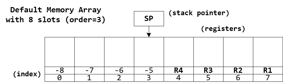
The default memory array contains eight slots 0 - 7. The last four slots are also accessible as Memory Registers via index aliases R1, R2, R3, and R4. A virtual Memory Stack starts at the index labeled SP and grows downward.
Memory arrays use modulo indexing allowing both positive and negative indices, as well as indices beyond the array end points which are aliased to slots within the array.
Memory array objects can be created with pyvgx.Memory() and passed to graph queries using the memory= query parameter. Queries will then use the supplied memory array instead of the default. The memory array is not initialized by the query and will remain after the query completes. A query may read and/or modify the memory array via one or more expressions in the query. The same memory object can be passed to subsequent queries for further processing.
Memory array objects are accessible from Python as regular list objects.
Memory array objects can have any size, only limited by system resources. Size is always a power of two, 2p where p is the array order.
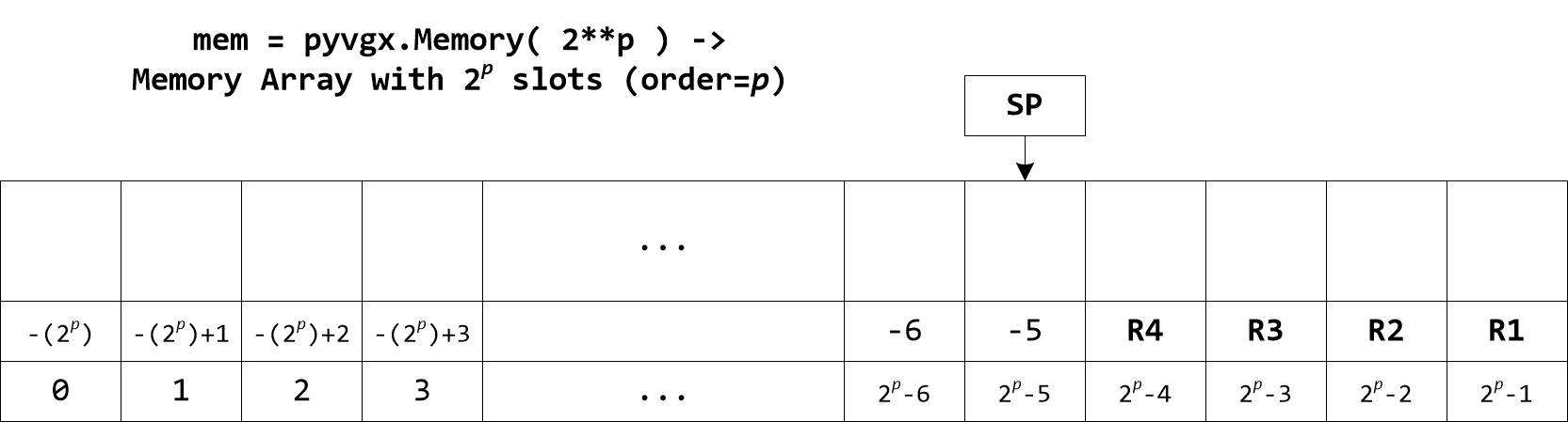
# Assumption: arc values are 0-99
# Create array with 100 slots (actual size will be 128)
mem = graph.Memory( 100 ) # size rounded up to nearest power of two
graph.Neighborhood(
    id     = "A",
    memory = mem,
    filter = "inc( int(.arc.value) )"
)
mem[0]  # freq of val=0
mem[1]  # freq of val=1
mem[2]  # freq of val=2
#...
mem[99] # freq of val=99
4.1. Memory Registers
The last four slots in a memory object are the registers R1 - R4. There is nothing special about these slots other than the convenience of being able to reference them in expressions using predefined index constants R1, R2, R3, and R4.
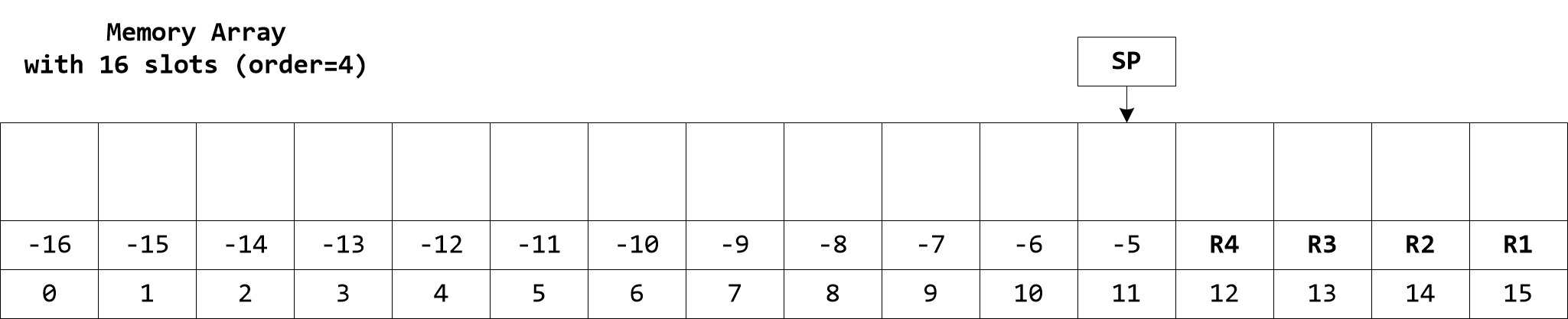
mem = graph.Memory( 16 )
graph.Evaluate( "store(R1, 111)", memory=mem )
graph.Evaluate( "store(R2, 222)", memory=mem )
mem[ R1 ]         # -> 111 (memory object as list)
mem.R1            # -> 111 (memory object attribute)
mem[ -1 ]         # -> 111 (indexing from end)
mem[ 15 ]         # -> 111 (indexing from start)
mem.R1 + mem.R2   # -> 333
graph.Evaluate( "load(R1)*load(R2)", memory=mem ) # -> 24642
To access the contents of a register it must be dereferenced using functions like load(), store(), etc., as shown in the example above. I.e. a constant like R1 is just the number -1 which represents a memory address.
|
4.2. Memory Stack
A virtual "stack" starts just below the registers and grows downward. A push operation puts a value on the stack and a pop operation removes a value from the stack and returns it. If the stack reaches the bottom of the array (index 0) it wraps around to the top overwriting register R1, then R2, etc. Likewise, repeated pop operations will move the stack pointer upwards wrapping to 0 when the last index is reached. Be careful to allocate a large enough array to accommodate the algorithm using it and to ensure balanced push and pop operations.
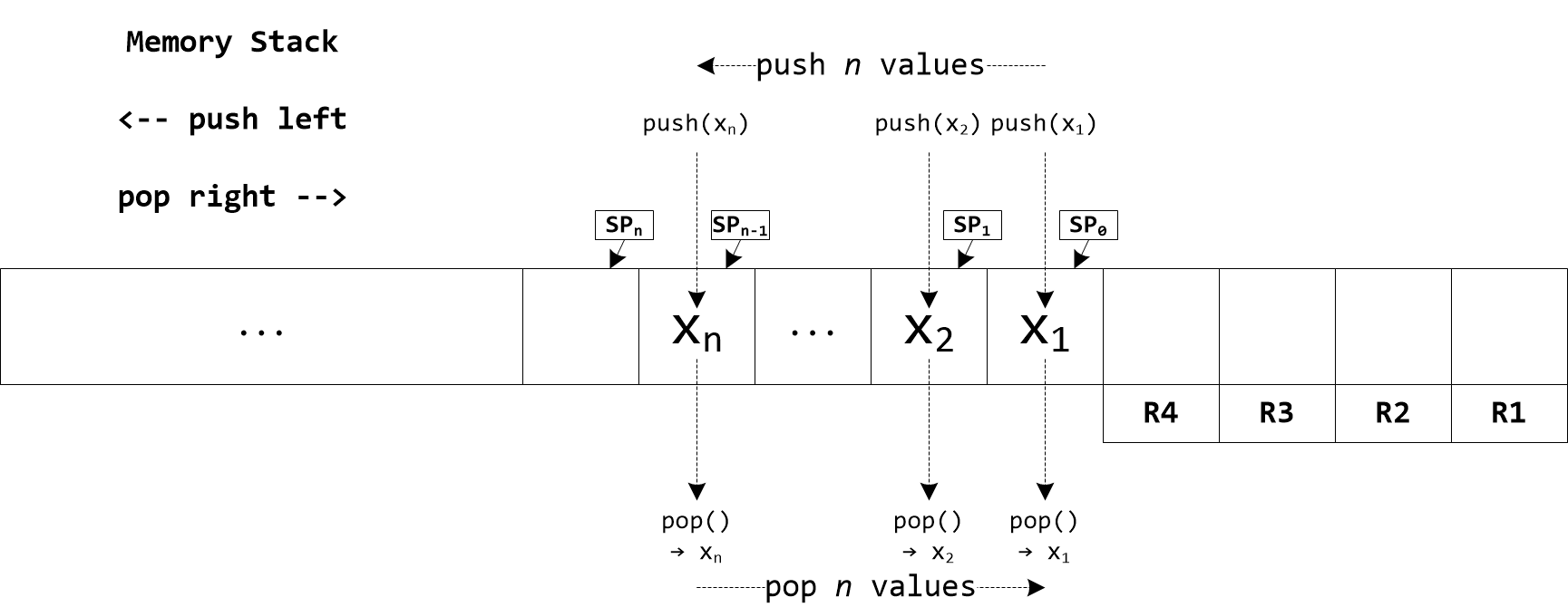
Using push and pop provides no protection against unbalanced calls. Make sure your algorithm is guaranteed to execute an equal number of each operation to avoid leaking the stack into other areas of the memory array you may be using for other purposes.
|
mem = graph.Memory( 16 )
graph.Evaluate( "push( 111 )", memory=mem )
graph.Evaluate( "push( 222 )", memory=mem )
graph.Evaluate( "push( 333 )", memory=mem )
mem[ 11 ]   # -> 111
mem[ 10 ]   # -> 222
mem[ 9 ]    # -> 333
graph.Evaluate( "pop()", memory=mem )   # -> 333
graph.Evaluate( "pop()", memory=mem )   # -> 222
graph.Evaluate( "pop()", memory=mem )   # -> 111
4.3. Memory Indexing
Memory arrays are modulo indexed, protecting system memory from invalid access and allowing negative indices to reference the array relative to its end. Although primarily included as a safeguard against invalid memory access you may find modulo indexing to be a useful feature when implementing certain algorithms.
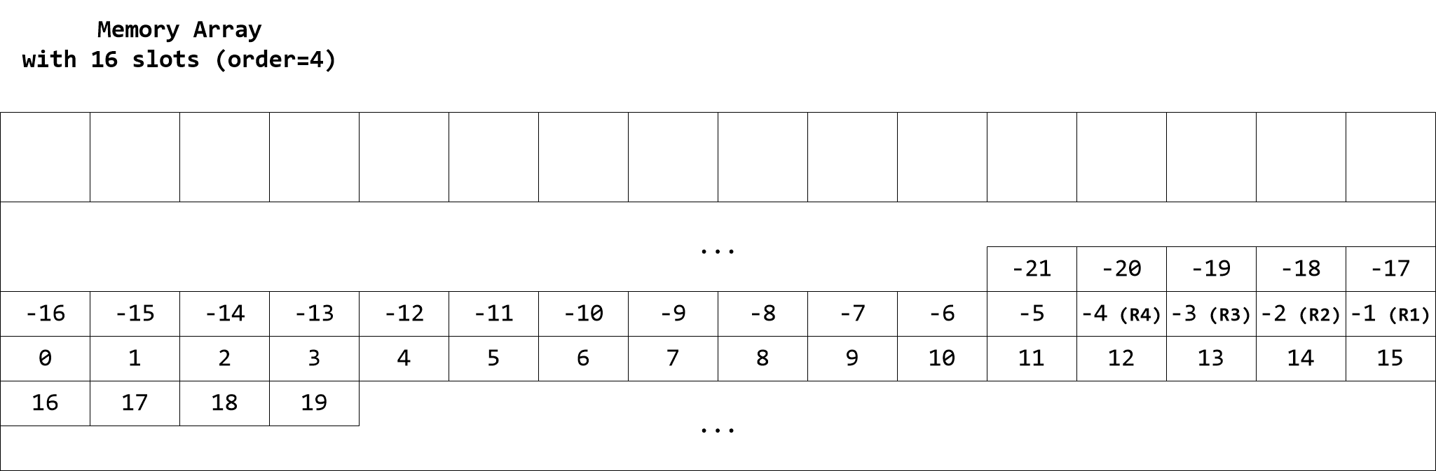
mem = graph.Memory( 16 )
graph.Evaluate( "store( 3, 555 )", memory=mem )
graph.Evaluate( "load( 3 )", memory=mem )    # ->   555
graph.Evaluate( "load( 19 )", memory=mem )    # ->   555
graph.Evaluate( "load( -13 )", memory=mem )     # ->   555
To restrict the indexing span to a sub-range of the array use the modindex() function to compute the array index.
|
4.4. Memory Python Interface for Assignment and Lookup
The Python interface for accessing pyvgx.Memory elements is similar to list. Lookup and assignment use the standard array subscript syntax [n] and slice syntax [a:b].
4.4.1. Memory Subscript
For subscript syntax [n] the behavior is the same as for list.
| Syntax | Python Value Type | Stored Value Type | Description |
|---|---|---|---|
|
int |
integer |
Assign an integer value to memory location n |
|
float |
real |
Assign a real value to memory location n |
|
str |
string |
Assign a string value to memory location n |
|
pyvgx.Vector |
vector |
Assign a vector object to memory location n |
|
[ int ] |
bitvector |
Assign integer value as a 64-bit bitvector to memory location n |
|
( int, float ) |
keyval |
Assign a keyval tuple to memory location n |
|
bytearray |
raw bytes |
Assign an array of raw (unsigned) bytes to memory location n |
|
bytes |
raw bytes (immutable) |
Assign an immutable array of (unsigned) bytes to memory location n |
| Syntax | When Stored Value Type Is… | Python Value Type | Description |
|---|---|---|---|
|
integer |
int |
Retrieve an integer value from memory location n as a Python int |
|
real |
float |
Retrieve a real value from memory location n as a Python float |
|
string |
str |
Retrieve a string value from memory location n as a Python str |
|
vector |
pyvgx.Vector |
Retrieve a vector object from memory location n as pyvgx.Vector |
|
bitvector |
[ int ] |
Retrieve a bitvector from memory location n as a Python list with a single int value |
|
keyval |
( int, float ) |
Retrieve a keyval from memory location n as a Python tuple with a 32-bit integer key and a single precision float value |
|
raw bytes |
bytearray |
Retrieve a sequence of raw bytes from memory location n as a Python bytearray object |
|
raw bytes |
bytes |
Retrieve an array of bytes from memory location n as a Python bytes object |
mem = graph.Memory(32)
mem[10] = 1234      # Assign 1234 to memory location 10
mem[11] = 3.14      # Assign 3.14 to memory location 11
mem[12] = "hello"   # Assign string "hello" to memory location 13
mem[13] = [0xFF00]  # Assign bitvector 0xFF00 to memory location 12
mem[14] = (42, 1.7) # Assign keyval 42:1.7 to memory location 14
mem[15] = bytearray( [10,20,0,0,50] ) # Assign raw bytes to mem 15
mem[16] = bytes( [1,2,3,4] ) # Assign raw bytes to mem 16
mem[17] = graph.sim.rvec(64) # Assign random vector to mem 17

# int
list( mem[10] )       # <class 'int'>
print( mem[10] )      # 1234
print( mem[-22] )     # 1234 (modulo indexing)

# float
type( mem[11] )       # <class 'float'>
print( mem[11] )      # 3.14

# str
type( mem[12] )       # <class 'str'>
print( mem[12] )      # hello

# bitvector
type( mem[13] )       # <class 'list'>
print( mem[13] )      # [65280]

# key/val
type( mem[14] )       # <class 'tuple'>
print( mem[14] )      # (42, 1.7000000476837158)

# bytearray
type( mem[15] )       # <class 'bytearray'>
list( mem[15] )       # [10, 20, 0, 0, 50]

# bytes
type( mem[16] )       # <class 'bytes'>
list( mem[16] )       # [1,2,3,4]

# vector
type( mem[17] )       # <class 'pyvgx.Vector'>
print( mem[17] )      # <PyVGX_Vector: ...>
4.4.2. Memory Slice
For slice syntax [a:b] the behavior is the same as for list with the exception of assignment which differs when the assignment list is smaller than the slice. The memory object is updated by applying the new values starting from the beginning of the slice and leaving the end of the slice unmodified. The behavior of list is to replace the entire slice with the new assigned values.
Just as for list slices may omit either end point, and negative indices reference backwards from the end.
| Syntax | Value Types | Description |
|---|---|---|
|
int → integer
|
Assign values v1 through vn to memory locations starting at a. If n < b - a the end of the memory slice remains unaffected. (This behavior is different from Python |
|
int ← integer
|
Return a list of values from memory locations a through b - 1. |
mem = graph.Memory(8)
mem[4:8] = [44,55,66,7.89]  # Assign multiple values to slice
mem[4:8] = [444,555]        # Partial slice assignment
print( mem[4:8] )           # [444, 555, 66, 7.89]

print( mem[:] )             # [0, 0, 0, 0, 444, 555, 66, 7.89]
print( mem[:5] )            # [0, 0, 0, 0, 444]
print( mem[3:] )            # [0, 444, 555, 66, 7.89]
print( mem[:-2] )           # [0, 0, 0, 0, 444, 555]
4.4.3. Memory Initialization
New memory objects can be initialized to specific values by passing an initializer list to the constructor. An existing memory object can have all its elements reset to a certain constant value or range of values.
# Construct using initializer
mem = graph.Memory( [100,1,1,1,50] )
# [100, 1, 1, 1, 50, 0, 0, 0]
len( mem ) # 8, smallest power of two to hold initializer

# Reset all elements to zero
mem.Reset()
# [0, 0, 0, 0, 0, 0, 0, 0]

# Reset all elements to 2.5
mem.Reset( 2.5 )
# [2.5, 2.5, 2.5, 2.5, 2.5, 2.5, 2.5, 2.5]

# Reset elements to a range
mem.Reset( 1, 5 ) # First value is 1, step is 5
# [1, 6, 11, 16, 21, 26, 31, 36]
4.4.4. Memory Sort
Memory objects can be sorted. It is possible to sort the entire array or a specific range within the array. The element comparator used for sorting is automatically chosen by the type of the first element in the range to be sorted.
mem = graph.Memory( 32 )

# Randomize 16 elements 0 through 15
graph.Evaluate( "mrandomize(0,15)", memory=m )

# Sort 16-element range 0 through 15
mem.Sort( 0, 16 )

# Reverse sort
mem.Sort( 0, 16, reverse=True )

# Sort 28 non-register elements
mem.Sort()
4.4.5. A Note on Memory Value Types
Although memory objects internally can hold elements of any type supported by the evaluator engine, the only element types accessible by the Python interpreter are integer, real, string, bitvector, keyval, bytearray and bytes which map to Python types or objects int, float, str, [int], (int,float), bytearray and bytes, respectively. Element types null, nan and inf in memory objects are accessed by the Python interpreter as Python type float with values nan, nan and inf, respectively.
- integer
-
Maps directly to Python
intmem[0] = 123 graph.Evaluate( "isint(load(0))", memory=mem ) # -> true mem[0] # -> 123 - real
-
Maps directly to Python
floatmem[1] = 3.14 graph.Evaluate( "isreal(load(1))", memory=mem ) # -> true mem[1] # -> 3.14 - string
-
This type is interpreted differently in different contexts. When accessing a Python memory object the evaluator string type maps directly to Python
strwith implicit UTF-8 encoding internally. When the evaluator engine executes an expression the string type also encompasses the bytearray and bytes types, i.e. the execution engine treats bytearray and bytes as subtypes of string.mem[2] = 'hello' g.Evaluate( "isstr(load(2))", memory=mem ) # -> true mem[2] # -> 'hello' - bitvector
-
This is a pseudo-type represented by a single-element Python
listwhere the element is a Pythonint. Bitvectors are assigned asmem[n] = [bv]. When retrieving the bitvector value it is returned as a singleton list[bv]. Evaluator expressions can also assign bitvectors, e.g."store( 0, bitvector( 0xFF00 ) )".mem[3] = [0xfff] graph.Evaluate( "isbitvector(load(3))", memory=mem ) # -> true mem[3] # -> [4095] - keyval
-
This is a pseudo-type represented by a two-element Python
tuplewhere the first element is a Pythonintand the second element is a Pythonfloat. Keyval items are assigned asmem[n] = (key, value). Note that key has a 32-bit range and value is truncated to single precision internally.mem[4] = (123,3.14) graph.Evaluate( "iskeyval(load(4))", memory=mem ) # -> true mem[4] # -> 123, 3.140000104904175) - bytearray and bytes
-
These types are applicable only when interacting with memory objects from Python. The Python
bytearrayandbytestypes are internally represented as subtypes of string, which means that evaluator expressions operate on all string data as arrays of bytes. When assigning to a memory location asmem[n] = bytearray( … )ormem[n] = bytes( … )the internal object is string with attributes indicating the subtype.mem[5] = bytearray([1,2,3]) graph.Evaluate( "isbytearray(load(5))", memory=mem ) # -> true graph.Evaluate( "isstr(load(5))", memory=mem ) # -> true mem[5] # -> bytearray(b'\x01\x02\x03') mem[6] = bytes([1,2,3]) graph.Evaluate( "isbytes(load(6))", memory=mem ) # -> true graph.Evaluate( "isstr(load(6))", memory=mem ) # -> true mem[6] # -> b'\x01\x02\x03' - null, nan, inf
-
These types indicating "no value" in various contexts are all interpreted as Python
floatwhen retrieved from memory objects. They cannot be set from Python.graph.Evaluate( "store(7,null)", memory=mem ) # -> None type(mem[7]) # -> <class 'float'> mem[7] # -> nan graph.Evaluate( "store(8,nan)", memory=mem ) # -> nan type(mem[8]) # -> <class 'float'> mem[8] # -> nan graph.Evaluate( "store(9,inf)", memory=mem ) # -> inf type(mem[9]) # -> <class 'float'> mem[9] # -> inf - vector
-
Maps directly to Python
pyvgx.Vectormem[10] = g.sim.rvec(128) g.Evaluate( "isvector(load(10))", memory=mem ) # -> true mem[10] # -> '<PyVGX_Vector: typ=euclidean len=128 mag=6.948...'
4.4.6. A note about strings and vectors in evaluator expressions
|
String and vector objects can be assigned to memory locations from within expressions and from the Python interpreter. The String and vector objects are retained by the If a memory instance is long-lived manual cleanup of strings and vectors is required to avoid unbounded buildup of objects that are no longer in use. Cleanup is performed explicitly via Note that copying existing strings or vectors between memory locations does not create new instances or additional ownership when performed by an expression. For instance, |
mem = graph.Memory( 16 )

mem[0] = 0xFF0000     # Type is integer
mem[1] = [ 0xFF0000 ] # Type is bitvector
mem[2] = 3.14         # Type is real
mem[3] = "Alice"      # Type is string
mem.R1 = graph.sim.rvec(64) # Type is vector
mem.R2 = graph.sim.rvec(64) # Type is vector

mem[0]                # -> 16711680
mem[1]                # -> [16711680]
mem[2]                # -> 3.14
mem[3]                # -> 'Alice'
mem.R1                # -> <PyVGX_Vector: ...>
mem.R2                # -> <PyVGX_Vector: ...>

graph.Evaluate( "isbitvector( load(0) )", memory=mem ) # -> 0
graph.Evaluate( "isbitvector( load(1) )", memory=mem ) # -> 1
graph.Evaluate( "mul( 2, 10 )", memory=mem )           # -> 31.4
graph.Evaluate( "load( 3 ) == 'Ali*'  ", memory=mem )  # -> 1
graph.Evaluate( "store( 4, 'Bob' )", memory=mem )      # -> 'Bob'
graph.Evaluate( "mov( 5, 3 )", memory=mem )            # -> 'Alice'
graph.Evaluate( "mov( 6, 4 )", memory=mem )            # -> 'Bob'
graph.Evaluate( "isvector(r1)", memory=mem )           # -> 1
graph.Evaluate( "cosine(r1,r2)", memory=mem )          # -> 0.02157

# Strings 'Alice' and 'Bob', and vectors are now deleted
graph.Evaluate( "mreset()", memory=mem )
5. Memory Operation Reference
5.1. Notation Conventions
The following notation is used to describe operations listed in all tables below.
| This notation is for describing how functions work, and has no relation to expression syntax. |
- Simple Assignment
:= -
The simple assignment operator
:=assigns the right operand to the left operand. For example, to indicate assignment of value x to memory location a we write[ a ] := x. - Operator Assignment
<op>= -
When the value of a left operand is modified by the right operand the general
<op>=syntax is used, such as+=,/=,>>=, etc. For example[ addr ] /= xmeans the value at location addr is divided by x and the result written back to location addr. - Exchange
:=: -
The exchange operator
:=:swaps the two operands. For example,[ a ] :=: [ b ]means the values at memory locations a and b are swapped. - Dereference
[] -
Dereference notation
[ addr ]is used to represent the contents at memory address addr. - Double Dereference
[[]] -
Double dereference notation
[[ addr ]]is used to represent the contents at address stored at address addr. For example,[[ a ]] := xmeans the value x is written to memory location stored in location a. As a concrete example, ifa = 1000and the value50is stored in location1000then[[ a ]] = 7will assign7to location50. - Range Dereference
[:] -
Dereference notation
[ a : b ]is used to indicate the contents of a range of addresses starting at address a and ending at address b, both endpoints included. For example, to assign value x to all memory locations starting at a and ending at b we write[ a : b ] := xWhen the right operand is or includes a range the right element i is assigned to left element i. For example,[ a : b ] := operation( [ a : b ] )means the operation is applied to each element starting at location a and ending at location b.
Operations taking a memory range input are inclusive of the end index. (This is different from how ranges are processed by the Python interpreter, where the end index is not included.) Negative indices are allowed. They count backwards from the element just beyond the end of the memory array, i.e. index -1 references the very last element.
|
5.2. Operations on Single Memory Locations
| Category | Functions |
|---|---|
|
|
|
|
|
|
|
|
|
|
|
|
|
|
|
|
|
|
|
5.2.1. Storing and Loading
| Function | Operation | Ret | Description |
|---|---|---|---|
Store |
|||
[dest] := x |
[dest] |
Assign numeric value x to memory location dest and return x |
|
[[ pdest ]] := x |
[[ pdest ]] |
Assign numeric value x to memory location pointed to by address in pdest and return x |
|
[dest] := x if cond == true |
cond |
If cond is nonzero assign numeric value x to memory location dest. Always returns cond. |
|
[[ pdest ]] := x if cond == true |
cond |
If cond is nonzero assign numeric value x to memory location pointed to by address in pdest. Always returns cond. |
|
Write |
|||
[dest1 : destn] := x1, x2, …, xn |
n |
Assign n numeric values x1 through xn to a range of consecutive destinations starting at dest1. The number n of values to write equals the number of value arguments xi and therefore destn is implied. If the end of the memory array is reached during writing, the next destination will be index 0 and writing continues until all xi have been written. |
|
[dest1 : destn] := x1, …, xn if cond == true |
cond |
If cond is nonzero the remaining arguments are passed to |
|
[[pdest]++] := x1
|
n |
Assign n numeric values x1 through xn to a range of consecutive destinations starting at the index referenced by pdest, incrementing the index in pdest after each iteration. If the end of the memory array is reached during writing, modulo indexing ensures the next destination will be index 0 and writing continues until all xi have been written. The value in pdest will have been incremented by n after the operation completes. |
|
If cond is true then:
|
cond |
If cond is nonzero the remaining arguments are passed to |
|
Load |
|||
[src] |
[src] |
Return value at memory location src |
|
[[ psrc ]] |
[[ psrc ]] |
Return value at memory location pointed to by psrc |
|
5.2.2. Stack
| Function | Operation | Ret | Description |
|---|---|---|---|
[stackptr] := x, stackptr −= 1 |
x |
Push numeric value x onto stack and return x |
|
if cond == true then
|
cond |
If cond is nonzero push numeric value x onto stack. Always returns cond. |
|
stackptr += 1, x := [stackptr] |
x |
Pop value from stack and return it |
|
x := [stackptr] |
x |
Return value at top of stack without popping |
5.2.3. Moving Data
| Function | Operation | Ret | Description |
|---|---|---|---|
Copy |
|||
[dest] := [src] |
[dest] |
Copy the value at memory location src into memory location dest and return the copied value |
|
[[ pdest ]] := [[ psrc ]] |
[[ pdest ]] |
Copy the value at memory location pointed to by address in psrc into memory location pointed to by address in pdest and return the copied value |
|
[dest] := [src]
|
cond |
If cond is nonzero copy the value at memory location src into memory location dest. Always returns cond. |
|
[[ pdest ]] :=[[ psrc ]]
|
cond |
If cond is nonzero copy the value at memory location pointed to by address in psrc into memory location pointed to by address in pdest. Always returns cond. |
|
Exchange |
|||
[m1] :=: [m2] |
[m1] |
Exchange the values at memory locations m1 and m2 and return the value at location m1 after the exchange (i.e. the value originally in m2) |
|
[[ pm1 ]] :=: [[ pm2 ]] |
[[ pm1 ]] |
Exchange the values at memory locations pointed to by addresses in pm1 and pm2 and return the value at location pointed to by address in pm1 after the exchange (i.e. the value originally pointed to by address in pm2) |
|
[m1] :=: [m2]
|
cond |
If cond is nonzero exchange the values at memory locations m1 and m2. Always returns cond. |
|
[[ pm1 ]] :=:[[ pm2 ]]
|
cond |
If cond is nonzero exchange the values at memory locations pointed to by addresses in pm1 and pm2. Always returns cond. |
|
5.2.4. Increment and Decrement
| Function | Operation | Ret | Description |
|---|---|---|---|
Increment |
|||
[dest] += 1 |
[dest] |
Increment value at memory location dest and return the new value |
|
[[ pdest ]] += 1 |
[[ pdest ]] |
Increment value at memory location pointed to by address in pdest and return the new value |
|
[dest] += 1 if cond == true |
cond |
If cond is nonzero increment value at memory location dest. Always returns cond. |
|
[[ pdest ]] += 1 if cond == true |
cond |
If cond is nonzero increment value at memory location pointed to by address in pdest. Always returns cond. |
|
Decrement |
|||
[dest] −= 1 |
[dest] |
Decrement value at memory location dest and return the new value |
|
[[ pdest ]] −= 1 |
[[ pdest ]] |
Decrement value at memory location pointed to by address in pdest and return the new value |
|
[dest] −= 1 if cond == true |
cond |
if cond is nonzero decrement value at memory location dest. Always returns cond. |
|
[[ pdest ]] −= 1 if cond == true |
cond |
if cond is nonzero decrement value at memory location pointed to by address in pdest. Always returns cond. |
|
5.2.5. Comparator
| Function | Operation | Ret | Description |
|---|---|---|---|
Equality |
|||
c := [a] == [b] |
c |
Return true if items in memory locations a and b compare equal, else return false |
|
c := [[ pa ]] == [[ pb ]] |
c |
Return true if items pointed to by addresses in memory locations pa and pb compare equal, else return false |
|
c := [a] != [b] |
c |
Return true if items in memory locations a and b compare not equal, else return false |
|
c := [[ pa ]] != [[ pb ]] |
c |
Return true if items pointed to by addresses in memory locations pa and pb compare not equal, else return false |
|
Greater |
|||
c := [a] > [b] |
c |
Return true if item in memory location a compares greater than item in memory location b, else return false |
|
c := [[ pa ]] > [[ pb ]] |
c |
Return true if item pointed to by address in memory location pa compares greater than item pointed to by address in memory location pb, else return false |
|
c := [a] >= [b] |
c |
Return true if item in memory location a compares greater than or equal to item in memory location b, else return false |
|
c := [[ pa ]] >= [[ pb ]] |
c |
Return true if item pointed to by address in memory location pa compares greater than or equal to item pointed to by address in memory location pb, else return false |
|
Less |
|||
c := [a] < [b] |
c |
Return true if item in memory location a compares less than item in memory location b, else return false |
|
c := [[ pa ]] < [[ pb ]] |
c |
Return true if item pointed to by address in memory location pa compares less than item pointed to by address in memory location pb, else return false |
|
c := [a] <= [b] |
c |
Return true if item in memory location a compares less than or equal to item in memory location b, else return false |
|
c := [[ pa ]] <= [[ pb ]] |
c |
Return true if item pointed to by address in memory location pa compares less than or equal to item pointed to by address in memory location pb, else return false |
|
5.2.6. Arithmetic
| Function | Operation | Ret | Description |
|---|---|---|---|
Addition |
|||
[addr] += x |
[addr] |
Add x to value at memory location addr and return the sum |
|
[addr] += x if cond == true |
cond |
If cond is nonzero add x to value at memory location addr. Always returns cond. |
|
Subtraction |
|||
[addr] −= x |
[addr] |
Subtract x from value at memory location addr and return the difference |
|
[addr] −= x if cond == true |
cond |
If cond is nonzero subtract x from value at memory location addr. Always returns cond. |
|
Multiplication |
|||
[addr] *= x |
[addr] |
Multiply value at memory location addr by x and return the product |
|
[addr] *= x if cond == true |
cond |
If cond is nonzero multiply value at memory location addr by x. Always returns cond. |
|
Division |
|||
[addr] /= x |
[addr] |
Divide value at memory location addr by x and return the quotient |
|
[addr] /= x if cond == true |
cond |
If cond is nonzero divide value at memory location addr by x. Always returns cond. |
|
Modulo |
|||
[addr] %= x |
[addr] |
Perform modulo by x operation on value at memory location addr and return the remainder |
|
[addr] %= x if cond == true |
cond |
If cond is nonzero perform modulo by x operation on value at memory location addr. Always returns cond. |
|
5.2.7. Bitwise
| Function | Operation | Ret | Description |
|---|---|---|---|
Shift |
|||
[addr] >>= b |
[addr] |
Shift value (interpreted as integer) at memory location addr right by b bits and return the new value. |
|
[addr] >>= b if cond == true |
cond |
If cond is nonzero shift value (interpreted as integer) at memory location addr right by b bits. Always returns cond. |
|
[addr] <<= b |
[addr] |
Shift value (interpreted as integer) at memory location addr left by b bits and return the new value. |
|
[addr] <<= b if cond == true |
cond |
If cond is nonzero shift value (interpreted as integer) at memory location addr left by b bits. Always returns cond. |
|
Bitwise AND |
|||
[addr] &= x |
[addr] |
Perform bitwise-AND operation on value (interpreted as integer) at memory location addr using bit mask x and return the new value. |
|
[addr] &= x if cond == true |
cond |
If cond is nonzero perform bitwise-AND operation on value (interpreted as integer) at memory location addr using bit mask x. Always returns cond. |
|
Bitwise OR |
|||
[addr] |= x |
[addr] |
Perform bitwise-OR operation on value (interpreted as integer) at memory location addr using bit mask x and return the new value. |
|
[addr] |= x if cond == true |
cond |
If cond is nonzero perform bitwise-OR operation on value (interpreted as integer) at memory location addr using bit mask x. Always returns cond. |
|
Bitwise XOR |
|||
[addr] ^= x |
[addr] |
Perform bitwise-XOR operation on value (interpreted as integer) at memory location addr using bit mask x and return the new value. |
|
[addr] ^= x if cond == true |
cond |
If cond is nonzero perform bitwise-XOR operation on value (interpreted as integer) at memory location addr using bit mask x. Always returns cond. |
|
5.2.8. Vector Arithmetic
| Function | Operation | Ret | Description |
|---|---|---|---|
\( y := \mathbf{A} \cdot \mathbf{B} \)
|
float( y ) |
Compute the dot-product of vectors A and B represented by bytearrays. Vector lengths must be equal, and a multiple of w bytes where w depends on the function version. Vector elements are interpreted as signed bytes.
|
|
\( y := \cos{ \theta } = \displaystyle \frac{ \mathbf{A} \cdot \mathbf{B}}{ \|\mathbf{A}\| \cdot \|\mathbf{B}\|} \)
|
y |
Compute cosine of angle \( \theta \) between vectors A and B (represented by bytearrays) whose lengths must be equal, and a multiple of w bytes where w depends on the function version. Vector elements are interpreted as signed bytes.
|
|
\( y := d( \mathbf{A}, \mathbf{B} ) = \displaystyle \|\overrightarrow{ \mathbf{AB} }\| \)
|
y |
Compute the Euclidean (L2) norm of the difference between vectors A and B represented by bytearrays. The number of vector dimensions must be a multiple of w bytes where w depends on the function version. Vector elements are interpreted as signed bytes.
|
|
\( y := hamdist( \mathbf{A}, \mathbf{B} ) \)
|
y |
Compute the Hamming Distance between the 64-bit fingerprints (LSH) of vectors A and B (represented by bytearrays or vector objects.) Vector elements are interpreted as signed bytes.
|
|
The However, there is a cost to using the Benchmarking is the only way to select the most performant vector function in a given application. |
5.2.9. Various Functions
| Function | Operation | Ret | Description |
|---|---|---|---|
[addr] += α · ( x − [addr] ) |
[addr] |
Update value at memory location addr from new value x using exponential smoothing factor α and return the updated value. |
|
[addr] += 1 |
[addr] |
Evaluate any number of sub-expressions <exprk> (discarding their return values), increment value at memory location addr and return the new value. This provides a way to count the number of times an expression is evaluated and to execute expressions that don’t contribute directly to the overall expression result value, but may be needed for their side-effects such as operating on memory locations that will be used later. |
|
[addr] += 1 if cond == true |
[cond] |
Same behavior as |
5.2.10. Indexing
| Function | Operation | Ret | Description |
|---|---|---|---|
x = i % mod + ofs |
x |
Compute the array index x for a sub-array index i defined by mod and ofs. |
|
[vertex.bitindex] |= vertex.bitvector |
1 or 0 |
Add vertex to memory array bitvector index by setting the appropriate bit of the value in a memory location determined by the vertex address |
|
[vertex.bitindex] & vertex.bitvector |
1 or 0 |
Test if vertex has been indexed in the memory array |
|
[vertex.bitindex] &= ~vertex.bitvector |
0 |
Remove vertex from memory array bitvector index by clearing the appropriate bit of the value in a memory location determined by the vertex address |
5.3. Operations on Multiple Memory Locations
These operations affect ranges of memory locations.
5.3.1. Function Naming Conventions
- Prefix
m* -
All functions of this type start with the letter
m. - Prefix
mi* -
Some functions are optimized for use with integer arrays and have the
miprefix. These functions have undefined behavior on non-integer data. - Prefix
mr* -
Some functions are optimized for use with floating point arrays and have the
mrprefix. These functions have undefined behavior on non-floating point data. - Prefix
mv* -
Some functions operate element-wise on two equally sized vectors and have the
mvprefix.
5.3.2. Array Indexing and Range Specification
- Array index subscript convention
-
Array indices are specified using 1-based offsets. The array A with k elements has its first element at A1 and its last element at Ak.
- Start and end indices
-
Functions that specify a memory range using start and end indices are inclusive of the end index. In general, a function
m<func>( m1, mn[, … ] )applies to memory locations m1, m2, …, mn. - Array location and length
-
Functions that specify a memory range using an array location A and its length k generally have the form
m<func>( A, k[, … ] )and apply to memory locations A1, A2, …, Ak.
5.3.3. Applying Operations to Memory Range
The simplified notation \( M_n \) is sometimes used to represent the set of n values in consecutive memory range m1 through mn.
\( M_n ::=\ [ m_1 : m_n ] \),
where dereference notation \( [m] \) is used to represent the value in memory location m.
Using this definition of \( M_n \) we can then describe functions more compactly.
| Function Example | Operation | Description |
|---|---|---|
|
\( M_n := f( M_n ) \)
|
Let \( y = f(x) \) and let \( [ m ] \) represent the value in memory location m. This evaluator function then computes \( y_i = f(x_i) \text{ for all } x_i = [m_i]\),
|
|
\( M_n := M_n \text{ <g> } p \)
|
Let \( y = g(x,p) \) and let \( [ m ] \) represent the value in memory location m. This evaluator function then computes \( y_i = g(x_i,p) \text{ for all } x_i = [m_i]\),
|
5.3.4. Section Links
| Category | Functions |
|---|---|
|
|
|
|
|
|
|
|
|
|
|
|
|
|
|
|
|
|
|
|
|
|
|
|
|
5.3.5. Set and Copy
| Function | Operation | Ret | Description |
|---|---|---|---|
\( M_n := x \) |
n |
Assign numeric value x to all memory locations m1 to mn and return the number of memory locations set. |
|
\( [ 0 : -1 ] := 0 \) |
n |
Set all memory locations to integer 0 and free all temporary string memory consumed by any previous calls to string functions such as |
|
\( M_n := \text{random}() \) |
n |
Assign a different random value in the range [0.0 - 1.0] to each memory location m1 to mn and return the number of memory locations affected. |
|
\( M_n := \text{randbits}() \) |
n |
Assign a different random bit pattern to each memory location m1 to mn and return the number of memory locations affected. |
|
\( [D_1 : D_k] := [S_1 : S_k] \) |
k |
Copy the contents of k consecutive source locations starting at S1 to the range of consecutive destinations starting at D1. If any Di or Si references a slot beyond the end of the memory array nothing is copied. The number of copied memory locations is returned. |
|
\( [ [pD] : [pD] + (k-1) ] := [ S_1 : S_k] \)
|
k |
Copy the contents of k consecutive source locations starting at S1 to the range of consecutive destinations starting at the memory location referenced by value in location pD, then increment the value stored in location pD by k. If any Si or the value at pD plus i - 1 references a slot beyond the end of the memory array nothing is copied. The number of copied memory locations is returned. |
|
\( [D_1 : D_n] := [obj_1 : obj_n] \)
|
n |
Copy the n raw quadwords of object obj into memory starting at location D1. The number of quadwords n comprising obj is determined automatically. If any Di references a slot beyond the end of the memory array nothing is copied. |
|
\( [m] := \text{null} \) |
m |
Set element at memory location m to null. |
|
\( \text{max}(k) \text{ such that} \)
|
k |
Return the number of elements between memory location A1 and the first occurrence of a null value or the end of the memory object if no null value is encountered. |
5.3.6. Heap Operations
These functions implement binary heap operations useful for maintaining subsets of smallest or largest values from a greater set of candidates.
The min and max versions of these functions signify min-heap or max-heap semantics. Recall that a min-heap will discard smaller values as larger values are added, and that a max-heap will discard larger values as smaller values are added:
- min-heap
-
Keep larger values
- max-heap
-
Keep smaller values
| Function | Operation | Ret | Description |
|---|---|---|---|
Initialize |
|||
\( [A_1 : A_k] := \text{null} \) |
k |
Prepare array of k elements starting at location A for use with heap operations. The array is initialized with null-values that are interpreted as inf for max-heaps and -inf for min-heaps. The array satisfies both shape property and heap property for binary min and max heaps after this. |
|
\( \text{heapifymin}( [ A_1 : A_k ] ) \) |
k |
Process array of k elements starting at location A such that the array satisfies the heap property for a min-heap. |
|
\( \text{heapifymax}( [ A_1 : A_k ] ) \) |
k |
Process array of k elements starting at location A such that the array satisfies the heap property for a max-heap. |
|
Populate |
|||
\(\text{if } [A_1] < x\ \text{, then}\)
|
1 or 0 |
Attempt to insert numeric value x into binary min-heap represented by array of k elements starting at location A and return 1 if successful. Inserting a new value implies discarding the previous smallest value from the heap (if no null-values remain). If the new value is less than all values in the heap nothing is inserted and 0 is returned. |
|
\(\text{if } [A_1] > x\ \text{, then}\)
|
1 or 0 |
Attempt to insert numeric value x into binary max-heap represented by array of k elements starting at location A and return 1 if successful. Inserting a new value implies discarding the previous largest value from the heap (if no null-values remain). If the new value is greater than all values in the heap nothing is inserted and 0 is returned. |
|
\(\text{for all } x_i, i \in \{1,2,...,n\}\)
|
N |
Attempt to insert numeric values x1 through xn into binary min-heap represented by array of k elements starting at location A and return the number of values inserted. This is functionally equivalent to calling |
|
\(\text{for all } x_i, i \in \{1,2,...,n\}\)
|
N |
Attempt to insert numeric values x1 through xn into binary max-heap represented by array of k elements starting at location A and return the number of values inserted. This is functionally equivalent to calling |
|
\(\text{for all } i \in \{1,2,...,n\}\)
|
n |
Process all numeric values in memory locations m1 through mn by attempting to insert them into binary min-heap represented by array of k elements starting at location A and return the number of processed values, whether inserted or not. On completion the array A will contain the k largest values from the source range. |
|
\(\text{for all } i \in \{1,2,...,n\}\)
|
n |
Process all numeric values in memory locations m1 through mn by attempting to insert them into binary max-heap represented by array of k elements starting at location A and return the number of processed values, whether inserted or not. On completion the array A will contain the k smallest values from the source range. |
|
5.3.7. Sorting
| Function | Operation | Ret | Description |
|---|---|---|---|
sortascending( [ A1 : Ak ] ) |
n ≤ k |
Sort array of k values starting at location A in ascending order, in-place. Any null-value compares greater-than any numeric value, and will appear at the end of the sorted array. The number n of non-null values is returned. (All other non-real elements are interpreted as integers.) |
|
sortdescending( [ A1 : Ak ] ) |
n ≤ k |
Sort array of k values starting at location A in descending order, in-place. Any null-value compares less-than any numeric value, and will appear at the end of the sorted array. The number n of non-null values is returned. (All other non-real elements are interpreted as integers.) |
|
sortascending( [ A1 : Ak ] )
|
k |
Sort array of k values (interpreted as floating point) starting at location A in ascending order, in-place. |
|
sortdescending( [ A1 : Ak ] )
|
k |
Sort array of k values (interpreted as floating point) starting at location A in descending order, in-place. |
|
reverse( [A1 : Ak] ) |
k |
Reverse array of k objects starting at location A, in-place. |
5.3.8. Type Cast
| Function | Operation | Ret | Description |
|---|---|---|---|
\( M_n := \text{integer}( M_n ) \) |
n |
Cast all values in memory locations m1 to mn to integer and return the number of memory locations affected by the operation. |
|
\( M_n := \text{integer}( \lfloor M_n \rceil ) \) |
n |
Cast all values in memory locations m1 to mn to integer after rounding to the nearest whole number and return the number of memory locations affected by the operation. |
|
\( M_n := \text{real}( M_n ) \) |
n |
Cast all values in memory locations m1 to mn to floating point and return the number of memory locations affected by the operation. |
|
\( M_n := \text{real}( M_n ) \) |
n |
Cast all values in memory locations m1 to mn to floating point and return the number of memory locations affected by the operation. |
5.3.9. Increment and Decrement
| Function | Operation | Ret | Description |
|---|---|---|---|
Increment |
|||
\( M_n := M_n + 1 \) |
n |
Increment all values in memory locations m1 to mn and return the number of memory locations affected by the operation. |
|
\( M_n := M_n + 1 \) |
n |
Increment all values in memory locations m1 to mn (interpreted as integers) and return the number of memory locations affected by the operation. |
|
\( M_n := M_n + 1 \) |
n |
Increment all values in memory locations m1 to mn (interpreted as floating point) and return the number of memory locations affected by the operation. |
|
Decrement |
|||
\( M_n := M_n - 1 \) |
n |
Decrement all values in memory locations m1 to mn and return the number of memory locations affected by the operation. |
|
\( M_n := M_n - 1 \) |
n |
Decrement all values in memory locations m1 to mn (interpreted as integers) and return the number of memory locations affected by the operation. |
|
\( M_n := M_n - 1 \) |
n |
Decrement all values in memory locations m1 to mn (interpreted as floating point) and return the number of memory locations affected by the operation. |
|
5.3.10. Arithmetic
| Function | Operation | Ret | Description |
|---|---|---|---|
Add |
|||
\( M_n := M_n + x \) |
n |
Add x to all values in memory locations m1 to mn and return the number of memory locations affected by the operation. |
|
\( M_n := M_n + x \) |
n |
Add integer x to all values in memory locations m1 to mn (interpreted as integers) and return the number of memory locations affected by the operation. |
|
\( M_n := M_n + x \) |
n |
Add floating point value x to all values in memory locations m1 to mn (interpreted as floating point) and return the number of memory locations affected by the operation. |
|
[ A1 : Ak ] := [ A1 + B1 : Ak + Bk ] |
k |
For all i from 1 through k, add numeric values in memory locations Ai and Bi and store the result in location Ai, then return k. |
|
Subtract |
|||
\( M_n := M_n - x \) |
n |
Subtract x from all values in memory locations m1 to mn and return the number of memory locations affected by the operation. |
|
\( M_n := M_n - x \) |
n |
Subtract integer x from all values in memory locations m1 (interpreted as integers) to mn and return the number of memory locations affected by the operation. |
|
\( M_n := M_n - x \) |
n |
Subtract floating point value x from all values in memory locations m1 to mn (interpreted as floating point) and return the number of memory locations affected by the operation. |
|
[ A1 : Ak ] := [ A1 − B1 : Ak − Bk ] |
k |
For all i from 1 through k, subtract numeric value in memory location Bi from numeric value in memory location Ai and store the result in location Ai, then return k. |
|
Multiply |
|||
\( M_n := M_n \cdot x \) |
n |
Multiply all values in memory locations m1 to mn by x and return the number of memory locations affected by the operation. |
|
\( M_n := M_n \cdot x \) |
n |
Multiply all values in memory locations m1 to mn (interpreted as integers) by integer x and return the number of memory locations affected by the operation. |
|
\( M_n := M_n \cdot x \) |
n |
Multiply all values in memory locations m1 to mn (interpreted as floating point) by floating point value x and return the number of memory locations affected by the operation. |
|
[ A1 : Ak ] := [ A1 * B1 : Ak * Bk ] |
k |
For all i from 1 through k, multiply numeric values in memory locations Ai and Bi and store the result in location Ai, then return k. |
|
Divide |
|||
\( M_n := \displaystyle \frac{M_n}{x} \) |
n |
Divide all values in memory locations m1 to mn by x and return the number of memory locations affected by the operation. |
|
\( M_n := \displaystyle \frac{M_n}{x} \) |
n |
Divide all values in memory locations m1 to mn (interpreted as integers) by integer x and return the number of memory locations affected by the operation. |
|
\( M_n := \displaystyle \frac{M_n}{x} \) |
n |
Divide all values in memory locations m1 to mn (interpreted as floating point) by floating point value x and return the number of memory locations affected by the operation. |
|
[ A1 : Ak ] := [ A1 / B1 : Ak / Bk ] |
k |
For all i from 1 through k, divide numeric value in memory location Ai by numeric value in memory location Bi and store the result in location Ai, then return k. |
|
Modulo |
|||
\( M_n := M_n \mod x \) |
n |
Perform modulo by x operation on all values in memory locations m1 to mn and return the number of memory locations affected by the operation. |
|
\( M_n := M_n \mod x \) |
n |
Perform integer modulo by x on all values in memory locations m1 to mn (interpreted as integers) and return the number of memory locations affected by the operation. |
|
\( M_n := M_n \mod x \) |
n |
Perform floating point modulo by x on all values in memory locations m1 to mn (interpreted as floating point) and return the number of memory locations affected by the operation. |
|
[ A1 : Ak ] := [ A1 % B1 : Ak % Bk ] |
k |
For all i from 1 through k, perform [Ai] modulo [Bi] and store the result in location Ai, then return k. |
|
Inverse |
|||
\( M_n := \displaystyle \frac{1}{M_n} \) |
n |
Perform the inverse operation on all values in memory locations m1 to mn and return the number of memory locations affected by the operation. |
|
\( M_n := \displaystyle \frac{1}{M_n} \) |
n |
Perform the inverse operation on all values in memory locations m1 to mn interpreted as floating point values and return the number of memory locations affected by the operation. |
|
Power |
|||
\( M_n := (M_n)^y \) |
n |
Raise all values in memory locations m1 to mn to the yth power and return the number of memory locations affected by the operation. |
|
\( M_n := (M_n)^y \) |
n |
Raise all values (interpreted as floating point values) in memory locations m1 to mn to the yth power and return the number of memory locations affected by the operation. |
|
Square |
|||
\( M_n := (M_n)^2 \) |
n |
Square all values in memory locations m1 to mn and return the number of memory locations affected by the operation. |
|
\( M_n := (M_n)^2 \) |
n |
Square all values (interpreted as floating point values) in memory locations m1 to mn and return the number of memory locations affected by the operation. |
|
Square Root |
|||
\( M_n := \displaystyle \sqrt{M_n} \) |
n |
Take the square root of all values in memory locations m1 to mn and return the number of memory locations affected by the operation. |
|
\( M_n := \displaystyle \sqrt{M_n} \) |
n |
Take the square root of all values (interpreted as floating point values) in memory locations m1 to mn and return the number of memory locations affected by the operation. |
|
5.3.11. Numeric
| Function | Operation | Ret | Description |
|---|---|---|---|
Ceil |
|||
\( M_n := \lceil M_n \rceil \) |
n |
Set all values in memory locations m1 to mn to their floating point values representing the smallest integers greater than or equal to their values. Return the number of memory locations affected by the operation. |
|
\( M_n := \lceil M_n \rceil \) |
n |
Set all values (interpreted as floating point values) in memory locations m1 to mn to their floating point values representing the smallest integers greater than or equal to their values. Return the number of memory locations affected by the operation. |
|
Floor |
|||
\( M_n := \lfloor M_n \rfloor \) |
n |
Set all values in memory locations m1 to mn to their floating point values representing the largest integers less than or equal to their values. Return the number of memory locations affected by the operation. |
|
\( M_n := \lfloor M_n \rfloor \) |
n |
Set all values (interpreted as floating point values) in memory locations m1 to mn to their floating point values representing the largest integers less than or equal to their values. Return the number of memory locations affected by the operation. |
|
Round |
|||
\( M_n := \lfloor M_n \rceil \) |
n |
Round all values in memory locations m1 to mn to the real values representing their nearest integers and return the number of memory locations affected by the operation.
|
|
\( M_n := \lfloor M_n \rceil \) |
n |
Round all values (interpreted as floating point values) in memory locations m1 to mn to the real values representing their nearest integers and return the number of memory locations affected by the operation. |
|
Absolute Value |
|||
\( M_n := | M_n | \) |
n |
Convert all values in memory locations m1 to mn to their absolute values and return the number of memory locations affected by the operation. |
|
\( M_n := | M_n | \) |
n |
Convert all values (interpreted as floating point) in memory locations m1 to mn to their absolute values and return the number of memory locations affected by the operation. |
|
Sign |
|||
\( M_n := \sgn(M_n) \)
|
n |
Replace all values in memory locations m1 to mn with their signs as 1 or -1, and return the number of memory locations affected by the operation. |
|
\( M_n := \sgn(M_n) \) |
n |
Replace all values (interpreted as floating point) in memory locations m1 to mn with their signs as 1.0 or -1.0, and return the number of memory locations affected by the operation. |
|
5.3.12. Logarithms and Exponential Functions
| Function | Operation | Ret | Description |
|---|---|---|---|
log2 |
|||
\( M_n := \log_2(M_n) \) |
n |
Compute the base-2 logarithm of values in memory locations m1 to mn. Return the number of memory locations affected by the operation. |
|
\( M_n := \log_2(M_n) \) |
n |
Compute the base-2 logarithm of values (interpreted as floating point) in memory locations m1 to mn. Return the number of memory locations affected by the operation. |
|
Natural Logarithm |
|||
\( M_n := \ln(M_n) \) |
n |
Compute the natural logarithm of values in memory locations m1 to mn. Return the number of memory locations affected by the operation. |
|
\( M_n := \ln(M_n) \) |
n |
Compute the natural logarithm of values (interpreted as floating point) in memory locations m1 to mn. Return the number of memory locations affected by the operation. |
|
log10 |
|||
\( M_n := \log_{10}(M_n) \) |
n |
Compute the base-10 logarithm of values in memory locations m1 to mn. Return the number of memory locations affected by the operation. |
|
\( M_n := \log_{10}(M_n) \) |
n |
Compute the base-10 logarithm of values (interpreted as floating point) in memory locations m1 to mn. Return the number of memory locations affected by the operation. |
|
exp2 |
|||
\( M_n := 2^{M_n} \) |
n |
Perform 2x for all values x in memory locations m1 to mn and return the number of memory locations affected by the operation. |
|
\( M_n := 2^{M_n} \) |
n |
Perform 2x for all values x (interpreted as floating point values) in memory locations m1 to mn and return the number of memory locations affected by the operation. |
|
Exponentiation |
|||
\( M_n := e^{M_n} \) |
n |
Perform ex for all values x in memory locations m1 to mn and return the number of memory locations affected by the operation. |
|
\( M_n := e^{M_n} \) |
n |
Perform ex for all values x (interpreted as floating point values) in memory locations m1 to mn and return the number of memory locations affected by the operation. |
|
exp10 |
|||
\( M_n := 10^{M_n} \) |
n |
Perform 10x for all values x in memory locations m1 to mn and return the number of memory locations affected by the operation. |
|
\( M_n := 10^{M_n} \) |
n |
Perform 10x for all values x (interpreted as floating point values) in memory locations m1 to mn and return the number of memory locations affected by the operation. |
|
5.3.13. Trigonometric and Hyperbolic
| Function | Operation | Ret | Description |
|---|---|---|---|
Angle Conversion |
|||
\( M_n := \displaystyle \frac{\pi}{180} \cdot M_n \) |
n |
Convert all values (assumed to be degrees) in memory locations m1 to mn to radians and return the number of memory locations affected by the operation. |
|
\( M_n := \displaystyle \frac{\pi}{180} \cdot M_n \) |
n |
Convert all values (assumed to be degrees and interpreted as floating point) in memory locations m1 to mn to radians and return the number of memory locations affected by the operation. |
|
\( M_n := \displaystyle \frac{180}{\pi} \cdot M_n \) |
n |
Convert all values (assumed to be radians) in memory locations m1 to mn to degrees and return the number of memory locations affected by the operation. |
|
\( M_n := \displaystyle \frac{180}{\pi} \cdot M_n \) |
n |
Convert all values (assumed to be radians and interpreted as floating point) in memory locations m1 to mn to degrees and return the number of memory locations affected by the operation. |
|
Trigonometric |
|||
|
\( M_n := \sin(M_n) \)
|
n |
Compute sin(x), cos(x) or tan(x) for all x in memory locations m1 to mn and return the number of memory locations affected by the operation. |
|
\( M_n := \sin(M_n) \)
|
n |
Compute sin(x), cos(x) or tan(x) for all x (interpreted as floating point) in memory locations m1 to mn and return the number of memory locations affected by the operation. |
Inverse Trigonometric |
|||
|
\( M_n := \arcsin(M_n) \)
|
n |
Compute asin(x), acos(x) or atan(x) for all x in memory locations m1 to mn and return the number of memory locations affected by the operation. |
|
\( M_n := \arcsin(M_n) \)
|
n |
Compute asin(x), acos(x) or atan(x) for all x (interpreted as floating point) in memory locations m1 to mn and return the number of memory locations affected by the operation. |
Hyperbolic |
|||
|
\( M_n := \sinh(M_n) \)
|
n |
Compute sinh(x), cosh(x) or tanh(x) for all x in memory locations m1 to mn and return the number of memory locations affected by the operation. |
|
\( M_n := \sinh(M_n) \)
|
n |
Compute sinh(x), cosh(x) or tanh(x) for all x (interpreted as floating point) in memory locations m1 to mn and return the number of memory locations affected by the operation. |
Inverse Hyperbolic |
|||
|
\( M_n := \arcsinh(M_n) \)
|
n |
Compute asinh(x), acosh(x) or atanh(x) for all x in memory locations m1 to mn and return the number of memory locations affected by the operation. |
|
\( M_n := \arcsinh(M_n) \)
|
n |
Compute asinh(x), acosh(x) or atanh(x) for all x (interpreted as floating point) in memory locations m1 to mn and return the number of memory locations affected by the operation. |
Sinc |
|||
|
\( M_n := \displaystyle \frac{\sin{ \pi M_n }}{\pi M_n} \) |
n |
Compute sin( πx ) / πx for all x in memory locations m1 to mn and return the number of memory locations affected by the operation. |
|
\( M_n := \displaystyle \frac{\sin{ \pi M_n }}{\pi M_n} \) |
n |
Compute sin( πx ) / πx for all x (interpreted as floating point) in memory locations m1 to mn and return the number of memory locations affected by the operation. |
5.3.14. Bitwise Operations
| Function | Operation | Ret | Description |
|---|---|---|---|
Shift |
|||
\( M_n := M_n \text{ >> } b \)
|
n |
Shift all values in memory locations m1 to mn right by b bits and return the number of memory locations affected by the operation. |
|
[ A1 : Ak ] := [ A1 >> B1 : Ak >> Bk ] |
k |
For all i from 1 through k, shift integer value in memory location Ai right by the number of bits indicated by integer value in memory location Bi and store the result in location Ai, then return k. |
|
\( M_n := M_n \text{ << } b \)
|
n |
Shift all values in memory locations m1 to mn left by b bits and return the number of memory locations affected by the operation. |
|
[ A1 : Ak ] := [ A1 << B1 : Ak << Bk ] |
k |
For all i from 1 through k, shift integer value in memory location Ai left by the number of bits indicated by integer value in memory location Bi and store the result in location Ai, then return k. |
|
Logical |
|||
\( M_n := M_n \text{ & } x \)
|
n |
Perform bitwise-AND operation on all values in memory locations m1 to mn using mask x and return the number of memory locations affected by the operation. |
|
[ A1 : Ak ] := [ A1 & B1 : Ak & Bk ] |
k |
For all i from 1 through k, perform bitwise-AND on integer values in memory locations Ai and Bi and store the result in location Ai, then return k. |
|
\( M_n := M_n \text{ | } x \)
|
n |
Perform bitwise-OR operation on all values in memory locations m1 to mn using mask x and return the number of memory locations affected by the operation. |
|
[ A1 : Ak ] := [ A1 | B1 : Ak | Bk ] |
k |
For all i from 1 through k, perform bitwise-OR on integer values in memory locations Ai and Bi and store the result in location Ai, then return k. |
|
\( M_n := M_n \text{ ^ } x \)
|
n |
Perform bitwise-XOR operation on all values in memory locations m1 to mn using mask x and return the number of memory locations affected by the operation. |
|
[ A1 : Ak ] := [ A1 ^ B1 : Ak ^ Bk ] |
k |
For all i from 1 through k, perform bitwise-XOR on integer values in memory locations Ai and Bi and store the result in location Ai, then return k. |
|
Other |
|||
\( M_n := popcnt(M_n) \)
|
n |
Count the number of bits set to 1 for all values in memory locations m1 to mn, update all locations with their respective bit counts and return the number of memory locations affected. |
|
5.3.15. Hashing
| Function | Operation | Ret | Description |
|---|---|---|---|
\( M_n := h(M_n) \)
|
n |
Compute the 64-bit integer hash of all values in memory locations m1 to mn, update all locations with their hash value and return the number of memory locations affected. |
5.3.16. Aggregation
| Function | Operation | Ret | Description |
|---|---|---|---|
Sum |
|||
\([dest] := \displaystyle \sum M_n \) |
[dest] |
Add all numeric values in memory locations m1 through mn and assign the resulting sum to memory location dest as a real value then return the result. |
|
\([dest] := \displaystyle \sum M_n \) |
[dest] |
Add all values (interpreted as floating point) in memory locations m1 through mn and assign the resulting sum to memory location dest as a real value then return the result. |
|
\([dest] := \displaystyle \sum (M_n)^2 \) |
[dest] |
Add the square of all numeric values in memory locations m1 through mn and assign the resulting sum to memory location dest then return the result. |
|
\([dest] := \displaystyle \sum (M_n)^2 \) |
[dest] |
Add the square of all values (interpreted as floating point) in memory locations m1 through mn and assign the resulting sum to memory location dest then return the result. |
|
\([dest] := \displaystyle \sum \frac{1}{M_n} \) |
[dest] |
Add the inverse of all numeric values in memory locations m1 through mn and assign the resulting sum to memory location dest then return the result. |
|
\([dest] := \displaystyle \sum \frac{1}{M_n} \) |
[dest] |
Add the inverse of all values (interpreted as floating point) in memory locations m1 through mn and assign the resulting sum to memory location dest then return the result. |
|
Product |
|||
\([dest] := \displaystyle \prod M_n \) |
[dest] |
Multiply all numeric values in memory locations m1 through mn and assign the resulting product to memory location dest then return the result. |
|
\([dest] := \displaystyle \prod M_n \) |
[dest] |
Multiply all values (interpreted as floating point) in memory locations m1 through mn and assign the resulting product to memory location dest then return the result. |
|
Mean |
|||
\([dest] := \displaystyle \frac{1}{n} \sum M_n \) |
[dest] |
Compute the arithmetic mean (average) of all numeric values in memory locations m1 through mn and assign the result to memory location dest then return the result. |
|
\([dest] := \displaystyle \frac{1}{n} \sum M_n \) |
[dest] |
Compute the arithmetic mean (average) of all values (interpreted as floating point) in memory locations m1 through mn and assign the result to memory location dest then return the result. |
|
\([dest] := \displaystyle \left(\frac{1}{n} \sum {\frac{1}{M_n}} \right)^{-1} \) |
[dest] |
Compute the harmonic mean of all numeric values in memory locations m1 through mn and assign the result to memory location dest then return the result. |
|
\([dest] := \displaystyle \left(\frac{1}{n} \sum {\frac{1}{M_n}} \right)^{-1} \) |
[dest] |
Compute the harmonic mean of all values (interpreted as floating point) in memory locations m1 through mn and assign the result to memory location dest then return the result. |
|
\([dest] := \displaystyle \sqrt[n]{\prod{M_n}} \) |
[dest] |
Compute the geometric mean of all numeric values in memory locations m1 through mn and assign the result to memory location dest then return the result. |
|
\([dest] := \displaystyle \sqrt[n]{\prod{M_n}} \) |
[dest] |
Compute the geometric mean of all values (interpreted as floating point) in memory locations m1 through mn and assign the result to memory location dest then return the result. |
|
Deviation |
|||
\( [dest] := \displaystyle \sqrt{ \frac{1}{n} \displaystyle \sum_{i=1}^n {(x_i-\mu)^2} } \)
|
[dest] |
Compute the standard deviation of numeric values in memory locations m1 through mn and assign the result to memory location dest then return the result. |
|
\( [dest] := \displaystyle \sqrt{ \frac{1}{n} \displaystyle \sum_{i=1}^n {(x_i-\mu)^2} } \) |
[dest] |
Compute the standard deviation of values (interpreted as floating point) in memory locations m1 through mn and assign the result to memory location dest then return the result. |
|
\( [dest] := \exp \left(\displaystyle \sqrt{\displaystyle \frac{\displaystyle \sum_{i=1}^n{\left(\ln{\frac{x_i}{\mu_g}}\right)^2}}{n}}\right) \)
|
[dest] |
Compute the geometric standard deviation of numeric values in memory locations m1 through mn and assign the result to memory location dest then return the result. |
|
\( [dest] := \exp \left(\displaystyle \sqrt{\displaystyle \frac{\displaystyle \sum_{i=1}^n{\left(\ln{\frac{x_i}{\mu_g}}\right)^2}}{n}}\right) \) |
[dest] |
Compute the geometric standard deviation of values (interpreted as floating point) in memory locations m1 through mn and assign the result to memory location dest then return the result. |
|
5.3.17. Array Probing
| Function | Operation | Ret | Description |
|---|---|---|---|
Simple |
|||
\( [dest] := \max( M_n ) \) |
mk |
Find the largest value in memory locations m1 through mn and assign it to memory location dest, then return the location mk where the largest value was found. |
|
\( [dest] := \min( M_n ) \) |
mk |
Find the smallest value in memory locations m1 through mn and assign it to memory location dest, then return the location mk where the smallest value was found. |
|
\( y = \begin{cases} 1 & \quad \text{if value } \in M_n \\ 0 & \quad \text{if value } \notin M_n \end{cases} \) |
y |
Return 1 if value occurs in any memory location m1 through mn, otherwise return 0. |
|
\( y = | { x \in M_n : x = \text{value} } | \) |
y |
Return the number of times value occurs in memory location range m1 through mn. |
|
\( y = cmp( [ A_1 : A_k ], [ B_1 : B_k ] ) \)
|
y |
For all i from 1 through k, compare numeric values in memory locations Ai and Bi. Immediately return -1 at the first iteration where [Ai] < [Bi] or 1 at the first iteration where [Ai] > [Bi]. If [Ai] == [Bi] for all i return 0. If k is such that either A or B extends beyond the end of memory -1 is returned. |
|
\( y = cmp( [ A_1 : A_k ], [ B_1 : B_k ] ) \)
|
y |
For all i from 1 through k, compare numeric values in memory locations Ai and Bi using approximate matching for real values. Real values a and b compare equal when \( |a-b| < \varepsilon \). Immediately return -1 at the first iteration where [Ai] < [Bi] or 1 at the first iteration where [Ai] > [Bi]. If [Ai] == [Bi] for all i return 0. If k is such that either A or B extends beyond the end of memory -1 is returned. |
|
\( k = \min( i ), i \in [1,n] \text{ such that} \)
|
mk or -1 |
Return first memory location mk where value occurs in range m1 through mn. If value does not occur in specified range return -1. |
|
Subset |
|||
\( y = \begin{cases} 1 & \quad \text{if } P_k \in M_n \\ 0 & \quad \text{if } P_k \notin M_n \end{cases} \)
|
1 or 0 |
Return 1 if all values in probe memory location range p1 through pk occur in memory location range m1 through mn, otherwise return 0. |
|
\( y = \begin{cases} 1 & \quad \text{if } P_k \in obj \\ 0 & \quad \text{if } P_k \notin obj \end{cases} \)
|
1 or 0 |
Return 1 if all values in probe memory location range p1 through pk occur in obj, otherwise return 0. The object obj is either a numeric array or a map, i.e. an object for which isarray() or ismap() is true. If obj is a numeric array its values must be integers. |
|
5.4. Mappings and Sets
These functions operate on built-in maps and sets associated with memory objects.
|
The integer set and vertex set functions operate on the same internal set structure. Mixing |
5.4.1. Integer Set
The integer set is used to store and check existence of unique (32-bit) integer keys. Object key may be of any type, but its raw bit value (as produced by asbits(key)) is always implied and only the 32 lower bits are used.
Key 0xffffffff is reserved and cannot be used.
| Function | Return Value | Description |
|---|---|---|
\( y = \begin{cases} 1 & \quad \text{key added} \\ 0 & \quad \text{already exists} \\ -1 & \quad \text{error} \end{cases} \) |
Add key to set and return 1 if added or 0 if key already existed in the set. If the value could not be added -1 is returned. |
|
\( y = \begin{cases} 1 & \quad \text{key deleted} \\ 0 & \quad \text{does not exist} \end{cases} \) |
Delete key from set and return 1 if deleted or 0 if key did not exist in the set. |
|
\( y = \begin{cases} 1 & \quad \text{key exists} \\ 0 & \quad \text{does not exist} \end{cases} \) |
Return 1 if key exists in set, otherwise return 0. |
|
number of mapped keys |
Return the number of keys in set. |
|
number of removed keys |
Remove all keys from set and return the number of keys removed. |
5.4.2. Vertex Set
The vertex set is used to store and check existence of unique vertex instances.
| Function | Return Value | Description |
|---|---|---|
\( y = \begin{cases} 1 & \quad \text{vertex added} \\ 0 & \quad \text{already exists} \\ -1 & \quad \text{error} \end{cases} \) |
Add vertex to set and return 1 if added or 0 if vertex already existed in the set. If the vertex could not be added -1 is returned. |
|
\( y = \begin{cases} 1 & \quad \text{vertex deleted} \\ 0 & \quad \text{does not exist} \end{cases} \) |
Delete vertex from set and return 1 if deleted or 0 if vertex did not exist in the set. |
|
\( y = \begin{cases} 1 & \quad \text{vertex exists} \\ 0 & \quad \text{does not exist} \end{cases} \) |
Return 1 if vertex exists in set, otherwise return 0. |
|
number of vertices |
Return the number of vertices in set. |
|
number of vertices |
Remove all vertices from set and return the number of vertices removed. |
6. Special Purpose Operations
This section describes specialized operations for solving specific problems.
| Function | Description |
|---|---|
Compare array object to probe stored in memory range and compute match score |
|
Time-dependent arc values |
6.1. sumprodobj()
Compute the sum of products of all matching pairs of items in object obj and memory location range \( [p_1 : p_k] \).
The object obj is either a numeric array or a map. If obj is a numeric array its values must be integers.
The items to be matched are compared using key function \(K(x)\) which is either the integer key of keyval item x, or x itself if x is an integer.
The item value \( V(x) \) is either the float value of keyval item x, or 1.0 if x is an integer.
6.1.1. Syntax
msumprodobj( p1, pk, obj ) -> y
6.1.2. Parameters
| Parameter | Type | Description |
|---|---|---|
p1 |
integer |
First memory location of probe item |
pk |
integer |
Last memory location of probe item |
obj |
numeric array or map |
Numeric array objects are sequences of integers, such as vertex properties assigned as |
6.1.3. Return Value
This function returns a floating point value representing the sum of products of item values for all items that occur in both obj and memory range \( [p_1 : p_k] \).
6.1.4. Remarks
Items to be matched and whose values are contributing to the sum must be plain integers or keyval items.
Memory probe items are assigned to the memory object using the respective data type syntax.
- Integer item in memory probe location
-
m[i] = integer_valueItem key is the assigned integer, and item has implicit value 1.0.
- Keyval item in memory probe location
-
m[i] = (integer_key, float_value)Item key is the tuple’s integer_key, and item value is the tuple’s float_value.
from pyvgx import *
g = Graph("test")
m = g.Memory(16)

# Assign integer items
m[0] = 123          # key=123, val=1.0
m[1] = 456          # key=456, val=1.0
m[2] = 789          # key=789, val=1.0

# Assign keyval items
m[3] = (200, 2.718) # key=200, val=2.718
m[4] = (300, 3.142) # key=300, val=3.142
Objects are typically vertex properties and are assigned according to property assignment syntax.
- Numeric array in vertex property
-
V[prop] = [v1, v2, …]The item key of each integer vi is the integer itself, and the item has implicit value 1.0.
- Keyval map in vertex property
-
V[prop] = { k1:v1, k2:v2, … }The item key of each ki : vi pair is integer key ki, and the item value is float vi.
from pyvgx import *
g = Graph("test")
V = g.NewVertex( "V" )

# Assign array of three integers to property 'p1'
V['p1'] = [123, 456, 789]

# Assign map of two int:float items to property 'p2'
V['p2'] = {200:2.718, 300:3.142}
6.1.5. Formula
The return value s is computed as follows.
\( s = \displaystyle \sum_{i=1}^k{ \left[ V(p_i) \sum_{j=1}^n{ \bigg( V(x_j) \: \big| \: x_j \in obj \wedge M(p_i,x_j) \bigg) } \right] }\)
where
\( V(x) = \begin{cases} \text{value of x} & \quad \text{if x is keyval} \\ 1 & \quad \text{if x is integer} \end{cases} \)
and
\( M(a,b) = \begin{cases} true & \quad \text{if } K(a) = K(b) \\ false & \quad \text{if } K(a) \ne K(b) \end{cases} \)
and
\( K(x) = \begin{cases} \text{key of x} & \quad \text{if x is keyval} \\ x & \quad \text{if x is integer} \end{cases} \)
and
\( n = | obj | \)
6.1.6. Example
from pyvgx import *
g = Graph("test")
m = g.Memory(16)

# Vertex with array and map properties
#V = g.NewVertex("V")
V['p1'] = [123, 456, 789]
V['p2'] = {200:2.718, 300:3.142}

# Probe items
m[0] = 123
m[1] = 456
m[2] = 789
m[3] = (200, 2.718)
m[4] = (300, 3.142)

# Probe against numeric array object will
# match three integer items and
# return 3.0
g.Evaluate( "msumprodobj(0,4,next['p1'])", memory=m, head="V" )

# Probe against keyval map object will
# match two keyval items and
# return 17.26
g.Evaluate( "msumprodobj(0,4,next['p2'])", memory=m, head="V" )
6.2. probealtarray()
Test if all elements of a probe stored in memory range [p1, pn] exist in array object altarray and return a position-dependent and match-type dependent score. The array can have up to 16 elements. Array elements are dual-value integers, divided into a primary region and a secondary (alternative) region. For a probe element and an array element to match their primary regions must be equal, or their secondary regions must be equal. A probe element may also be a dual bitvector split into a primary and secondary region for cases where the probe is already known to match the array object in one or more positions, but needs to be included for keeping track of number of matches and their positions.
6.2.1. Syntax
probealtarray( p1, pn, altarray, prefix_boost, alt_deboost ) -> score
6.2.2. Parameters
| Parameter | Type | Description |
|---|---|---|
p1, pn |
2 x 32-bit integers
|
Memory locations 1, 2, …, n of the probe holding dual-value integers or dual bitvectors |
altarray |
Numeric array object (multi-valued vertex property) |
Array object to be probed, containing up to 16 dual-value integers. |
prefix_boost |
real |
Score multiplier for ordered match starting from the first element of altarray |
alt_deboost |
real |
Score multiplier for match involving one or more matches on secondary (alternative) element regions |
altarray: The values in altarray are presumed to be encoded as two 32-bit integers packed into a 64-bit integer. This special encoding will be referred to as dual-value integer. The upper 32 bits represent the primary region. The lower 32 bits represent the secondary (or alternative) region. This makes it possible for two distinct values to occupy the same position in altarray, enabling position-aware matching with alternative scoring depending on which region of the element is matched.
[p1, pn]: A probe element is either a dual-value integer encoded the same way as values in altarray, or a dual bitvector. A bitvector in this context uses only the 32 lower bits, subdivided into a 16-bit primary region (bits 16-31) and a 16-bit secondary region (bits 0-15.) A bitvector asserts a match in all position(s) of altarray corresponding to bitvector position(s) set to 1.
Probe elements p1 through pn reference a consecutive region of a memory object into which the probe data must be entered before calling probealtarray().
|
Probe bitvectors are limited to 32 bits and therefore dual bitvectors are limited to 16 bit positions. Hence the number of positions we are able to keep track of in altarray is also 16. The reason for the 32-bit restriction is to maintain compatibility with arc values, which often will be the carriers of data used to construct bitvector probes. |
6.2.3. Return Value
The default (un-boosted) score returned when all probe elements exist in the array is 1.0. If one or more probe elements do not exist in array 0.0 is returned.
If probe elements match the array in order, starting from the first array element (a prefix match) the return score is multiplied by prefix_boost.
If any element match occurs because of a match in the secondary region (due to no match in primary region) the return score is multiplied by alt_deboost.
6.2.4. Remarks
Probe elements p1 through pn are evaluated against values in altarray, in order. Each time a match is found it is "consumed", i.e. if a probe element matched position q in altarray no subsequent probe element can match position q in altarray.
Probe elements encoded as dual-value integers are compared against values in altarray by matching primary regions first, then secondary regions if no match in primary regions. As long as ordered (prefix) matches can continue to be made, an element is declared a match if either primary or secondary regions match. If ordered matching fails, unordered matching is attempted and in this case all possibilities for primary region matches are considered before any secondary region matches are considered.
Probe elements encoded as dual bitvectors are used to assert matches in altarray at the position(s) corresponding to 1s in the bitvectors. When a bitvector probe pk is matched against a value in altarray, the position q of the least significant 1 in the bitvector that also corresponds to unmatched position q in altarray (if one exists) is marked as matched, i.e. position q cannot be matched by any subsequent probe. The primary bit-region of pk is processed first, then if no match the secondary bit-region of pk is processed. Note that bitvector probe pk will only consume one position q in altarray even if pk has multiple bits set to 1.
6.2.5. Example
# Create a vertex and assign a multi-valued
# property of dual-value integers
V = graph.NewVertex( "V" )
V['data'] = [ (1111 << 32) + 555, (4444 << 32) + 444, (3333 << 32) + 1000, (7777 << 32) + 555 ]

# Create the probe
probe = graph.Memory( 32 )
probe[1] = (1111 << 32) + 555   # primary match (pos 0)
probe[2] = (9999 << 32) + 1000  # secondary match (pos 2)
probe[3] = [ 0x00000009 ]       # secondary match (pos 0 and 3)

# Execute search
graph.Evaluate( "probealtarray( 1 , 3, vertex['data'], 100.0, 0.5 )", head=V, memory=probe )  # -> 0.5

# Explanation:
# probe[1] has a primary match for 1111 in pos 0
# probe[2] has a secondary match for 1000 in pos 2
# probe[3] is a bitvector and asserts secondary matches
#          in positions 0 and 3 (0x9 = binary 1001). Position 0
#          was consumed by probe[1] but position 3 was not
#          yet consumed and therefore a match occurs.
# We do not have a prefix match, and we are falling back
# on secondary matches, hence the returned score is
# 1.0 * 0.5 = 0.5.
6.3. synarc.decay() and synarc.xdecay()
Compute age-dependent arc value.
- Linear decay
synarc.decay() -
\( N_t = N_0 - r \cdot t \)
- Exponential decay
synarc.xdecay() -
\( N_t = N_0 e^{-\lambda t} \)
6.3.1. Syntax
synarc.decay( relationship[, rate] ) # -> decayed_value Nt
synarc.xdecay( relationship[, rate] ) # -> decayed_value Nt
6.3.2. Parameters
| Parameter | Type | Default | Description |
|---|---|---|---|
relationship |
|
Relationship type given as string or as integer enumeration. To enable computation of decayed value Nt the relationship must be represented by a multiple arc comprising a creation ( |
|
rate |
|
\( \displaystyle \frac{1}{t_{end} - t_0} \) |
Optional rate overrides rate derived from arc timestamps. Decay constants are always computed as:
|
6.3.3. Return Value
This function returns either null or a real value:
- null
-
Evaluation of the expression containing
synarc.decay()orsynarc.xdecay()occurs for each traversed arc during neighborhood traversal, and for all such evaluations this function returns null. - Nt
-
Post-traversal evaluation of the expression takes place each time all arcs between two vertices have been processed, and at this point a real value representing decayed value Nt is returned.
6.3.4. Remarks
Arc decay functions are special in that they require multiple evaluations to compute a result. Arc components are first captured during traversal of the multiple arc, and finally the decayed value Nt is computed using those components when the expression is invoked one additional time post-traversal.
6.3.4.1. Capture arc components
During processing of arcs the arc decay functions will capture arc information for arcs whose relationship matches the rel argument. The arc’s value is captured and interpreted according to the modifier.
- t0
-
(A) -[ rel, M_TMC, tc ]-> (B)
(A) -[ rel, M_TMM, tm ]-> (B)When a decay function is evaluated at time t1 the creation (or modification) time t0 provides a reference for computing elapsed time t required by the decay formulas. If both
M_TMCandM_TMMarcs exist the value from theM_TMMarc takes precedence.\( t_0 = \begin{cases} t_m & \quad \text{if M_TMM arc exists} \\ t_c & \quad \text{if M_TMC arc exists and M_TMM arc does not exist} \end {cases} \)
If neither
M_TMCnorM_TMMarc exists t0 takes on a default value:\( t_0 = \begin{cases} t_{end} - \frac{1}{rate} & \quad \text{if rate > 0 and M_TMX arc exists} \\ graph.t_0 & \quad \text{if rate = 0 or M_TMX arc does not exist} \end {cases} \)
where \( graph.t_0 \) is the graph inception time.
- tend
-
(A) -[ rel, M_TMX, tx ]-> (B)The time t1 at which the arc’s decayed value reaches its minimum is tend, which is provided by an arc with the
M_TMXmodifier.\( t_{end} = t_x \)
If no arc with modifier
M_TMXexists tend takes on a default value:\( t_{end} = \begin{cases} t_0 + \frac{1}{rate} & \quad \text{if } rate > 0 \text{ and } t_0 > graph.t_0 \\ \to \infty & \quad \text{if } rate = 0 \text{ or } t_0 \leq graph.t_0 \end{cases} \)
- N0
-
(A) -[ rel, M_FLT, vi ]-> (B)
(A) -[ rel, M_ACC, vi ]-> (B)
(A) -[ rel, M_SIM, vi ]-> (B)
(A) -[ rel, M_DIST, vi ]-> (B)The arc’s initial value N0 is derived as the sum of all arcs with a floating point modifier. Let n be the number of such arcs, then:
\( N_0 = \begin{cases} \displaystyle \sum_{i=1}^n{v_i} & \quad \text{if } n > 0 \\ 1 & \quad \text{if } n = 0 \text{ and } rate > 0 \\ 0 & \quad \text{if } n = 0 \text{ and } rate = 0 \end{cases}\)
Arcs with relationships other than rel, or with modifiers other than those with timestamp or floating point values are ignored by the arc decay function. The ignored non-floating point modifiers are M_STAT, M_LSH, M_INT, M_UINT, and M_CNT.
The value returned by synarc.decay() and synarc.xdecay() is always null when the expression is evaluated as part of arc traversal.
6.3.4.2. Post-traversal evaluation
Arc decay functions are available for use in adjacency filters and traversal filters, i.e. filters involving processing of arcs. Normally such filters evaluate once for each arc. However, when an expression contains one or more calls to an arc decay function the expression is invoked one additional time for each head vertex following completion of arc processing for that head vertex. Specifically, if a arcs are processed for h head vertices the expression is invoked a + h times, instead of the normal a times for expressions without arc decay functions.
Beware of the extra evaluation per vertex pair since this will have side-effects for other functions within the same expression such as count(), inc(), rwrite(), and many others.
|
6.3.4.3. Synthetic arc and return value
The arc processed by the expression at the final invocation is a synthetic arc that triggers different behavior for functions like synarc.decay() and synarc.xdecay(). The behavior triggered is to compute and return the decayed value Nt based on the current time t1 and arc components captured during processing of arcs.
Expressions should check for next.arc.issyn == true or include a type-check such as isreal() on the value returned by synarc.decay() and synarc.xdecay() if the value is to be used as part of a larger expression.
6.3.4.4. Decay Formula Summary
- Elapse time t
-
The relative elapse time t is the difference between the expression invocation time t1 and the arc’s initial time t0.
\( t = t_1 - t_0 \)
- Decay rate
-
If rate is not explicitly given, it is derived from the arc’s lifespan:
\( rate = \displaystyle \frac{1}{t_{end} - t_0} \)
- Initial value
-
The arc’s initial value N0 is computed as:
\( N_0 = \displaystyle \sum_{i=1}^n{ v_i } \)
where n is the number of arc values v with a floating point modifier.If no arcs exist with a floating point modifier (n = 0) the initial value defaults to:
\( N_0 = \begin{cases} 1 & \quad \text{if } rate > 0 \\ 0 & \quad \text {if } rate = 0 \end{cases}\)
- Linear decay function
synarc.decay( rel[, rate] ) -
The arc value at elapse time t is computed as:
\( N_t = N_0 - r \cdot t \)
\( r = \begin{cases} \frac{N_0}{t_{end} - t_0} & \quad \text{if no rate parameter} \\ rate \cdot N_0 & \quad \text{if rate parameter specified} \end{cases} \)
- Exponential decay function
synarc.xdecay( rel[, rate] ) -
The arc value at elapse time t is computed as:
\( N_t = N_0 e^{-\lambda t} \)
\( \lambda = \begin{cases} \frac{ln\left( 10^4 \right)}{t_{end} - t_0} & \quad \text{if no rate parameter} \\ rate \cdot \ln\left( 10^4 \right) & \quad \text{if rate parameter specified} \end{cases} \)
|
When exponential decay constant λ is derived from the arc’s lifespan it is chosen such that Nt decays to 0.01% of the arc’s initial value N0 at t1 = tend. This also implies a decay to 10% of initial value 1/4 through the lifespan, 1% of initial value 1/2 through the lifespan, and 0.1% of initial value 3/4 through the lifespan. |
6.3.5. Returning decayed arc value in search result
Search results include arcs that are collected during graph traversal. Arcs are collected into the result set in accordance with the query collect parameter or the vertex condition 'traverse': { 'collect': … } clause. Values computed in evaluator expressions can also be collected but must be done using collect() or collectif() functions.
When collecting search results using evaluator expressions it is often desirable to collect using the C_SCAN mode. This mode disables automatic collection of traversed arcs and ensures traversal of the entire neighborhood.
|
To collect an arc with a decayed value we pass the result of synarc.decay() or synarc.xdecay() to collect().
6.3.5.1. Example: Collect decayed arc value
collect( synarc.decay( 'score' ) )The function collect( value ) works by adding the currently traversed arc to the search result with the arc’s value overridden by value, which in the above example is the decayed value. Note that collect( value ) does nothing unless value is numeric and therefore ignores the null return value from synarc.decay() during traversal (i.e. when arc components needed to compute the decayed value are captured.) Only the post-traversal evaluation step results in a numeric value and this is when the arc is collected.
The arc collected this way will appear in the result as:
-[ 'score', M_FLT, Nt ]->
6.3.6. Complete example
from pyvgx import *

# Build a small graph
g = Graph( "decaytest" )
g.Connect( "A", ("score", M_FLT, 100.0), "B", lifespan=3600 )
g.Connect( "A", ("score", M_FLT, 50.0),  "C", lifespan=3600 )
g.Connect( "A", ("score", M_FLT, 25.0),  "D", lifespan=86400 )

# Wait a few seconds...

# Query with LINEAR DECAY
g.Neighborhood( id      = "A",
                collect = C_SCAN,
                fields  = F_AARC,
                filter  = "collect( synarc.decay( 'score' ) )"
)
# [
#   ( A )-[ score <M_FLT> 99.8160 ]->( B ),
#   ( A )-[ score <M_FLT> 49.9080 ]->( C ),
#   ( A )-[ score <M_FLT> 24.9981 ]->( D )
# ]

# Wait some more...

# Query with EXPONENTIAL DECAY
g.Neighborhood( id      = "A",
                collect = C_SCAN,
                fields  = F_AARC,
                filter  = "collect( synarc.xdecay( 'score' ) )"
)
# [
#   ( A )-[ score <M_FLT> 43.6150 ]->( B ),
#   ( A )-[ score <M_FLT> 21.8075 ]->( C ),
#   ( A )-[ score <M_FLT> 24.1504 ]->( D )
# ]

# Query with EXPONENTIAL DECAY and override decay rate to emulate
# 15 minute lifespan of all arcs.
g.Neighborhood( id      = "A",
                collect = C_SCAN,
                fields  = F_AARC,
                filter  = "collect( synarc.xdecay( 'score', 1/900 ) )"
)
# [
#   ( A )-[ score <M_FLT> 0.0552536 ]->( B ),
#   ( A )-[ score <M_FLT> 0.0276268 ]->( C ),
#   ( A )-[ score <M_FLT> 0.0138134 ]->( D )
# ]